Adaptive transform for manifold-valued data

This package contains all software developed as part of Workpackage 2.1 (Adaptive transform for manifold-valued data) of the DEDALE project. For an in-depth description of this workpackage, we refer to the associated technical report.

The software consists of three main parts:

1. An implementation of the (bandlimited) α-shearlet transform (in AlphaTransform.py, in three versions:
   • A fully sampled (non-decimated), translation invariant, fast, but memory-consuming implementation
   • A fully sampled, translation invariant, slightly slower, but memory-efficient implementation
   • A subsampled (decimated), not translation invariant, but fast and memory-efficient implementation.
2. Implementations (in AdaptiveAlpha.py) of three criteria that can be used to adaptively choose the value of α, namely:
   • The asymptotic approximation rate (AAR),
   • the mean approximation error (MAE),
   • the thresholding denoising performance (TDP).
3. A chart-based implementation (in SphereTransform.py) of the α-shearlet transform for functions defined on the sphere.

In the following, we provide brief explanations and hands-on experiments for all of these aspects. The following table of content can be used for easy navigation:

Table of Contents

1. The α-shearlet transform: A crash course

2. Adaptively choosing α

   a) Asymptotic approximation rate (AAR)

   b) Mean approximation error (MAE)

   c) Thresholding denoising performance (TDP)

3. The α-shearlet transform for functions defined on the sphere

The α-shearlet transform: A crash course

The following demonstrates a very simple use case of the α-shearlet transform: We compute the transform of an example image, threshold the coefficients, reconstruct and compute the error. The code is longer than strictly necessary, since along the way give a demonstration of the general usage of the transform.

>>> # Importing necessary packages
>>> from AlphaTransform import AlphaShearletTransform as AST
>>> import numpy as np
>>> import matplotlib.pyplot as plt
>>> from scipy import misc

>>> im = misc.face(gray=True)
>>> im.shape
(768, 1024)

>>> # Setting up the transform
>>> trafo = AST(im.shape[1], im.shape[0], [0.5]*3) # 1
Precomputing shearlet system: 100%|███████████████████████████████████████| 52/52 [00:05<00:00,  8.83it/s]

>>> # Computing and understanding the α-shearlet coefficients
>>> coeff = trafo.transform(im) # 2
>>> coeff.shape # 3
(53, 768, 1024)
>>> trafo.indices # 4
[-1,
 (0, -1, 'r'), (0, 0, 'r'), (0, 1, 'r'),
 (0, 1, 't'), (0, 0, 't'), (0, -1, 't'),
 (0, -1, 'l'), (0, 0, 'l'), (0, 1, 'l'),
 (0, 1, 'b'), (0, 0, 'b'), (0, -1, 'b'),
 (1, -2, 'r'), (1, -1, 'r'), (1, 0, 'r'), (1, 1, 'r'), (1, 2, 'r'),
 (1, 2, 't'), (1, 1, 't'), (1, 0, 't'), (1, -1, 't'), (1, -2, 't'),
 (1, -2, 'l'), (1, -1, 'l'), (1, 0, 'l'), (1, 1, 'l'), (1, 2, 'l'),
 (1, 2, 'b'), (1, 1, 'b'), (1, 0, 'b'), (1, -1, 'b'), (1, -2, 'b'),
 (2, -2, 'r'), (2, -1, 'r'), (2, 0, 'r'), (2, 1, 'r'), (2, 2, 'r'),
 (2, 2, 't'), (2, 1, 't'), (2, 0, 't'), (2, -1, 't'), (2, -2, 't'),
 (2, -2, 'l'), (2, -1, 'l'), (2, 0, 'l'), (2, 1, 'l'), (2, 2, 'l'),
 (2, 2, 'b'), (2, 1, 'b'), (2, 0, 'b'), (2, -1, 'b'), (2, -2, 'b')]

>>> # Thresholding the coefficients and reconstructing
>>> np.max(np.abs(coeff)) # 5
2041.1017181588547
>>> np.sum(np.abs(coeff) > 200) / coeff.size # 6
0.020679905729473761
>>> thresh_coeff = coeff * (np.abs(coeff) > 200) # 7
>>> recon = trafo.inverse_transform(thresh_coeff, real=True) # 8
>>> np.linalg.norm(im - recon) / np.linalg.norm(im) # 9
0.13912540983541383

>>> plt.imshow(recon, cmap='gray')
<matplotlib.image.AxesImage object at 0x2b0f568c25c0>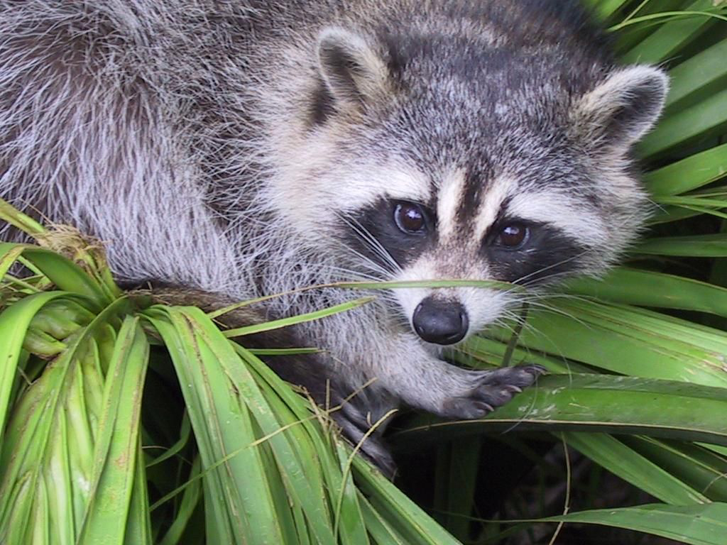
>>> plt.show()

Importing necessary packages

The first few (unnumbered) lines import relevant packages and load (a gray scale version of) the following test image, which has a resolution of 1024 x 768 pixels:

Setting up the transform

Then, in line 1, we create an instance trafo of the class AlphaShearletTransform (which is called AST above for brevity). During construction of this object, the necessary shearlet filters are precomputed. This may take some time (5 seconds in the example above), but speeds up later computations.

The three parameters passed to the constructor of trafo require some explanation:

• The first parameter is the width of the images which can be analyzed using the trafo object.

• Similarly, the second parameter determines the height.

• The third parameter is of the form [alpha] * N, where N determines the number of scales of the transform and alpha determines the value of α.

  The reason for this notation is that in principle, one can choose a different value of α on each scale. Since [0.5] * 3 = [0.5, 0.5, 0.5], one can use this notation to obtain a system using a single value of α across all scales.

All in all, we see that line 1 creates a shearlet system (i.e., α = 0.5) with 3 scale (plus a low-pass) for images of dimension 1024 x 768.

Computing and understanding the α-shearlet coefficients

Line 2 shows that the α-shearlet coefficients of the image im can be readily computed using the transform method of trafo. As seen in line 3, this results in an array of size 53, where each of the elements of the array is an array (an image) of size 1024 x 768, i.e., of the same size as the input image.

To help understand the meaning of each of these coefficient images coeff[i], for i = 0, ..., 52, the output of line 4 is helpful: Associated to each coefficient image coeff[i], there is an index trafo.indices[i] which encodes the meaning of the coefficient image, i.e., the shearlet used to compute it.

The special index -1 stands for the low-pass part. All other indices are of the form (j, k, c), where

• j encodes the scale. In the present case, j ranges from 0 to 2, since we have 3 scales.

• k encodes the amount of shearing, ranging from -⌈2^{j(1 - α)}⌉ to ⌈2^{j(1 - α)}⌉ on scale j.

• c encodes the cone to which the shearlet belongs (in the Fourier domain). Precisely, we have the following correspondence between the value of c and the corresponding frequency cones:

  value of c	'r'	't'	'l'	'b'
  Frequency cone	right	top	left	bottom

Note that if we divide the frequency plane into four cones, such that each shearlet has a real-valued Fourier transform which is supported in one of these cones, then the shearlets themselves (i.e., in space) can not be real-valued. Hence, if real-valued shearlets are desired, one can pass the constructor of the class AlphaShearletTransform the additional argument real=True. In this case, the frequency plane is split into a horizontal (encoded by 'h') and a vertical (encoded by 'v') cone, as is indicated by the following example:

>>> trafo_real = AST(im.shape[1], im.shape[0], [0.5]*3, real=True)
Precomputing shearlet system: 100%|██████████████████████████████████████| 26/26 [00:03<00:00,  5.62it/s]
>>> trafo_real.indices
[-1,
 (0, -1, 'h'), (0, 0, 'h'), (0, 1, 'h'),
 (0, 1, 'v'), (0, 0, 'v'), (0, -1, 'v'),
 (1, -2, 'h'), (1, -1, 'h'), (1, 0, 'h'), (1, 1, 'h'), (1, 2, 'h'),
 (1, 2, 'v'), (1, 1, 'v'), (1, 0, 'v'), (1, -1, 'v'), (1, -2, 'v'),
 (2, -2, 'h'), (2, -1, 'h'), (2, 0, 'h'), (2, 1, 'h'), (2, 2, 'h'),
 (2, 2, 'v'), (2, 1, 'v'), (2, 0, 'v'), (2, -1, 'v'), (2, -2, 'v')]

Thresholding the coefficients & reconstructing

When called without further parameters, the method trafo.transform computes a normalized transform, so that effectively all shearlets are normalized to have L² norm 1. With this normalization, line 5 shows that the largest coefficient has size about 2041. We now (arbitrarily) pick a threshold of 200 and see (in line 6) that only about 2% of the coefficients are larger than this threshold. Next, we set all coefficients which are smaller (in absolute value) than 200 to zero and save the resulting thresholded coefficients as thresh_coeff, in line 7.

In line 8, we then use the method inverse_transform of the trafo object to compute the inverse transform. Since we know that the original image was real-valued, we pass the additional argument real=True. This has the same effect as reconstructing without this additional argument and then taking the real part. Line 9 shows that the relative error is about 13.9%.

Finally, the last two lines display the reconstructed image.

Changes for the subsampled transform

Above, we showed how our implementation of the fully sampled α-shearlet transform can be used to compute the α-shearlet transform of an image and reconstruct (with thresholded coefficients). For the subsampled transform, this can be done very similarly; the main difference one has to keep in mind is that for the fully sampled transform, one obtains an array of "coefficient images" which are all of the same size. In contrast, due to the subsampling, the "coefficient images" for the subsampled transform are all of different sizes:

>>> from AlphaTransform import AlphaShearletTransform as AST
>>> import matplotlib.pyplot as plt
>>> import numpy as np
>>> from scipy import misc

>>> im = misc.face(gray=True)
>>> trafo = AST(im.shape[1], im.shape[0], [0.5]*3, subsampled=True) # 1
Precomputing shearlets: 100%|████████████████████████████████████████████| 52/52 [00:00<00:00, 69.87it/s]
>>> coeff = trafo.transform(im) # 2

>>> type(coeff).__name__ # 3
'list'
>>> [c.shape for c in coeff] # 4
[(129, 129),
 (364, 161), (364, 161), (364, 161),
 (97, 257), (97, 257), (97, 257),
 (364, 161), (364, 161), (364, 161),
 (97, 257), (97, 257), (97, 257),
 (514, 321), (514, 321), (514, 321), (514, 321), (514, 321),
 (193, 364), (193, 364), (193, 364), (193, 364), (193, 364),
 (514, 321), (514, 321), (514, 321), (514, 321), (514, 321),
 (193, 364), (193, 364), (193, 364), (193, 364), (193, 364),
 (727, 641), (727, 641), (727, 641), (727, 641), (727, 641),
 (385, 513), (385, 513), (385, 513), (385, 513), (385, 513),
 (727, 641), (727, 641), (727, 641), (727, 641), (727, 641),
 (385, 513), (385, 513), (385, 513), (385, 513), (385, 513)]

>>> np.max([np.max(np.abs(c)) for c in coeff]) # 5
2031.0471969998314
>>> np.sum([np.sum(np.abs(c) > 200) for c in coeff]) # 6
22357
>>> np.sum([np.sum(np.abs(c) > 200) for c in coeff]) / np.sum([c.size for c in coeff]) # 7
0.0023520267754635542
>>> thresh_coeff = [c * (np.abs(c) > 200) for c in coeff] # 8
>>> recon = trafo.inverse_transform(thresh_coeff, real=True) # 9
>>> np.linalg.norm(im - recon) / np.linalg.norm(im)
0.13945789596375507

Up to the first marked line, everything is identical to the code for the fully sampled transform. The only difference in line 1 is the additional argument subsampled=True to obtain a subsampled transform. Then, in line 2, the transform of the image im is computed just as for the fully sampled case.

The main difference to the fully sampled transform becomes visible in lines 3 and 4: In contrast to the fully sampled transform, where the coefficients are a 3-dimensional numpy array, the subsampled transform yields a list of 2-dimensional numpy arrays, with varying shapes. This shape is constant with respect to the shear k as long as the scale j and the cone c are kept fixed, but varies strongly with j and c. In face, for a quadratic image, the shape would only depend on the scale j.

Since we have a list of numpy arrays instead of a single numpy array, all operations on the coefficients are more cumbersome to write down (using list comprehensions), but are identical in spirit to the case of the fully sampled transform, cf. lines 5-8.

The actual reconstruction (in line 9) is exactly identical to the fully sampled case. It is interesting to note that only about 0.24% of the coefficients - and thus much less than the 2% for the fully sampled transform - are larger than the threshold. Nevertheless, the relative error is essentially the same.

Adaptively choosing α

In the following, we show for each of the three optimality criteria (AAR, MAE and TDP) how our implementation can be used to determine the optimal value of α for a given set of images.

Asymptotic approximation rate (AAR)

The following code uses a grid search to determine the value of α which yields the best asymptotic approximation rate (as described in the technical report) for the given set of images:

>>> from AdaptiveAlpha import optimize_AAR

>>> shearlet_args = {'real' : True, 'verbose' : False} # 1
>>> images = ['./Review/log_dust_test.npy'] # 2
>>> num_scales = 4 # 3
>>> num_alphas = 3 # 4

>>> optimize_AAR(images, num_scales, 1 / (num_alphas - 1), shearlet_args=shearlet_args)
First step: Determine the maximum relevant value...
alpha loop: 100%|████████████████████████████████████████████████████████| 3/3 [00:10<00:00,  3.48s/it]
image loop: 100%|████████████████████████████████████████████████████████| 1/1 [00:01<00:00,  1.60s/it]
Maximum relevant value: 0.04408709120918954

Second step: Computing the approximation errors...
alpha loop: 100%|████████████████████████████████████████████████████████| 3/3 [01:40<00:00, 30.99s/it]
Image loop: 100%|████████████████████████████████████████████████████████| 1/1 [00:46<00:00, 46.89s/it]
Thresh. loop: 100%|██████████████████████████████████████████████████████| 50/50 [00:45<00:00,  1.10it/s]

Third step: Computing the approximation rates...
Common breakpoints: [0, 4, 34, 50]
Last common linear part: [34, 50)

last slopes:
   alpha = 1.00 : -0.161932 + 0.012791
   alpha = 0.50 : -0.161932 + 0.000108
 * alpha = 0.00 : -0.161932 - 0.012900

Optimal value: alpha = 0.00

In addition to the output shown above, executing this code will display the following plot:

We now briefly explain the above code and output: In the short program above, we first import the function optimize_AAR which will do the actual work. Then, we define the parameters to be passed to this function:

1. In line 1, we determine the properties of the α-shearlet systems that will be used:

   • 'real': True ensures that real-valued shearlets are used.
   • 'verbose': False suppresses some output, e.g. the progress bar for precomputing the shearlet system.

   Another possible option would be 'subsampled': True if one wants to use the subsampled transform. Note though that this is incompatible with the 'real': True option.

2. In line 2, we determine the set of images that is to be used. To ensure fast computations, we only take a single image for this example. Specifically, the used image is the logarithm of one of the 12 faces of cosmic dust data provided by CEA, as depicted in the following figure:

   

3. The variable num_scales determines how many scales the α-shearlet systems should use.

4. Since we are using a grid search (i.e., we are only considering finitely many values of α), the variable num_alphas is used to determine how many different values of α should be distinguished. These are then uniformly spread in the interval [0,1]. Again, to ensure fast computations, we only consider three different values, namely α=0, α=0.5 and α=1.

Finally, we invoke the function optimize_AAR with the chosen parameters. As described in the technical report, this function does the following:

1. It determines a range [0, c₀] such that for c≥c₀, all α-shearlet transforms yield the same error when all coefficients of absolute value ≤c are set to zero ("thresholded").

2. It computes the reconstruction errors for the different values of α after thresholding the coefficients with a threshold of c₀·b^k for k=0,...,K-1.

   The default value is K=50. This can be adjusted by passing e.g. the argument num_x_values=40 as an additional argument to optimize_AAR. Likewise, the base b (with default value b=1.25) can be adjusted by passing e.g. base=1.3 as a further argument.

3. It determines a partition of {0, ..., K-1} into at most 4 intervals such that on each of these intervals, each of the (logarithmic) error curves is almost linear.

   In the example run above, the end points of the resulting partition are given by Common breakpoints: [0, 4, 34, 50]. In this case, the resulting partition has only three intervals instead of 4, since on each of these intervals, the best linear approximation is already sufficiently good.

4. For each value of α, the function then determines the slopes of the (logarithmic) error curve on the last of these intervals and compares these slopes.

   The optimal value of α (in this case α=0) is the one with the smallest slope, i.e., with the highest decay of the error. To allow for a visual comparison, optimize_AAR also displays a plot of the (logarithmic) error curves, including the partition into the almost linear parts.

Mean approximation error (MAE)

The following code uses a grid search to determine the value of α which yields the best mean approximation error (as described in the technical report) for the given set of images:

>>> from AdaptiveAlpha import optimize_MAE
>>> shearlet_args = {'real' : True, 'verbose' : False} # 1
>>> images = ['./Review/log_dust_test.npy'] # 2
>>> num_scales = 4
>>> num_alphas = 3
>>> optimize_MAE(images, num_scales, 1 / (num_alphas - 1), shearlet_args=shearlet_args)
First step: Determine the maximum relevant value...
alpha loop: 100%|████████████████████████████████████████████████████████| 3/3 [00:11<00:00,  3.61s/it]
image loop: 100%|████████████████████████████████████████████████████████| 1/1 [00:01<00:00,  1.61s/it]
Maximum relevant value: 0.006053772894213893

Second step: Computing the approximation errors...
alpha loop: 100%|████████████████████████████████████████████████████████| 3/3 [01:40<00:00, 31.13s/it]
image loop: 100%|████████████████████████████████████████████████████████| 1/1 [00:48<00:00, 48.25s/it]
thresholding loop: 100%|█████████████████████████████████████████████████| 50/50 [00:46<00:00,  1.08it/s]

Final step: Computing optimal value of alpha...
mean errors:
   alpha = 1.00 : +0.024105 + 0.000258
   alpha = 0.50 : +0.024105 + 0.000015
 * alpha = 0.00 : +0.024105 - 0.000273

Optimal value: alpha = 0.00

In addition to the output shown above, executing this code will display the following plot:

We now briefly explain the above code and output: In the short program above, we first import the function optimize_MAE which will do the actual work. Then, we define the parameters to be passed to this function:

1. In line 1, we determine the properties of the α-shearlet systems that will be used:

   • 'real': True ensures that real-valued shearlets are used.
   • 'verbose': False suppresses some output, e.g. the progress bar for precomputing the shearlet system.

   Another possible option would be 'subsampled': True if one wants to use the subsampled transform. Note though that this is incompatible with the 'real': True option.

2. In line 2, we determine the set of images that is to be used. To ensure fast computations, we only take a single image for this example. Specifically, the used image is the logarithm of one of the 12 faces of cosmic dust data provided by CEA, as depicted in the figure above.

3. The variable num_scales determines how many scales the α-shearlet systems should use.

4. Since we are using a grid search (i.e., we are only considering finitely many values of α), the variable num_alphas is used to determine how many different values of α should be distinguished. These are then uniformly spread in the interval [0,1]. Again, to ensure fast computations, we only consider three different values, namely α=0, α=0.5 and α=1.

Finally, we invoke the function optimize_MAE with the chosen parameters. As described in the technical report, this function does the following:

1. It determines a range [0, c₀] such that for c≥c₀, all α-shearlet transforms yield the same error when all coefficients of absolute value ≤c are set to zero ("thresholded").

2. It computes the reconstruction errors for the different values of α after thresholding the coefficients with a threshold of c = c₀·i / K for i = 0, ..., K-1.

   The default value is K=50. This can be adjusted by passing e.g. the argument num_x_values=40 as an additional argument to optimize_MAE.

3. For each value of α, the function then determines the mean of all these approximation errors. The optimal value of α (in this case α=0) is the one with the smallest mean approximation error.

   To allow for a visual comparison, optimize_MAE also displays a plot of the error curves.

Thresholding Denoising Performance (TDP)

In the following, we show how the denoising performance of an α-shearlet system can be used as an optimality criterion for adaptively choosing the correct value of α.

Since the (logarithmic) dust data used for the previous experiments does not allow for an easy visual comparison between the original image and the different denoised versions, we decided to instead use the following 684 x 684 cartoon image (taken from SMBC) as a toy example:

The following code uses a grid search over different values of α to determine the value with the optimal denoising performance:

>>> from AdaptiveAlpha import optimize_denoising

>>> image_paths=['./Review/cartoon_example.png']       # 1
>>> num_alphas = 3                                     # 2
>>> num_scales = 5                                     # 3
>>> num_noise_levels = 5                               # 4
>>> shearlet_args = {'real' : True, 'verbose' : False} # 5

>>> optimize_denoising(image_paths,
                       num_scales,
                       1 / (num_alphas - 1),
                       num_noise_levels,
                       shearlet_args=shearlet_args)
image loop: 100%|██████████████████████████████████████████████████████████| 1/1 [01:33<00:00, 93.16s/it]
alpha loop: 100%|██████████████████████████████████████████████████████████| 3/3 [01:33<00:00, 28.44s/it]
noise loop: 100%|██████████████████████████████████████████████████████████| 5/5 [00:46<00:00,  9.38s/it]

Averaged error over all images and all noise levels:
alpha = 1.00: 0.0961
alpha = 0.50: 0.0900
alpha = 0.00: 0.0948

Optimal value on whole set: alpha = 0.50

In addition to the output shown above, executing the sample code also displays the following plot:

We now briefly explain the above code and output: First, we import from AdaptiveAlpha.py the function optimize_denoising which will do the actual work. We then set the parameters to this function. In the present case, we want to

• analyze the cartoon image shown above,
• use α-shearlet transforms with real-valued shearlets (cf. line 5, the second part of that line suppresses some output),
• use α-shearlet transforms with 5 scales (line 4),
• use 5 different noise levels λ (line 4) which are uniformly spaced in [0.02, 0.4],
• compare three different values of α, which are uniformly spaced in [0,1], i.e, α=1, α=0.5 and α=0.

In more realistic experiment, one would of course use a larger set of test images and consider more different values of α, possibly also with a larger number of different noise levels. But here, we are mainly interested in a quick execution time, so we keep everything small.

Finally, we invoke the function optimize_denoising which - briefly summarized - does the following:

1. It normalizes each of the K x K input images to have L² norm equal to 1. Then, for each image, each value of α and each noise level λ in [0.02,0.4], a distorted image is calculated by adding artificial Gaussian noise with standard deviation σ=λ/K to the image.

   This standard deviation is chosen in such a way that the expected squared L² norm of the noise is λ².

   One can specify other ranges for the noise level than the default range [0.02, 0.4] by using the paramters noise_min and noise_max.

2. The α-shearlet transform of the distorted image is determined.

3. Hard thresholding is performed on the set of α-shearlet coefficients. The thresholding parameter (i.e., the cutoff value) c is chosen scale- and noise dependent via c = mσ, with m being a scale-dependent multiplier.

   Numerical experiments showed that good results are obtained by taking m=3 for all scales except the highest and m=4 for the highest scale. This is the default choice made in optimize_denoising. If desired, this default choice can be modified using the parameter thresh_multiplier.

4. The inverse α-shearlet transform of the thresholded coefficients is determined and the L²-error between this reconstruction and the original image is calculated.

5. The optimal value of α is the one for which the L²-error averaged over all images and all noise levels is the smallest.

The plot which is displayed by optimize_denoising depicts the mean error over all images as a function of the employed noise level λ for different values of α. In the present case, we are only considering one image (N=1). Clearly, shearlets (i.e., α=0.5) turn out to be optimal for our toy example.

For an eye inspection, optimize_denoising also saves the noisy image and the reconstructions for the largest noise level (λ=0.4) and the different α values to the current working directory. A small zoomed part of these reconstructions - together with the same part of the original image and the noisy image - can be seen below:

original image

noisy image

α=0

α=0.5

α=1

The α-shearlet transform for functions defined on the sphere

As described in the technical report, we use a chart-based approach for computing the α-shearlet transform of functions defined on the sphere. Precisely, we use the charts provided by the HEALPix pixelization of the sphere, which divides the sphere into 12 faces and provides cartesian charts for each of these faces. The crucial property of this pixelization is that each pixel has exactly the same spherical area.

Now, given a function f defined on the sphere (in a discretized version, as a so-called HEALPix map), one can use the function get_all_faces() from SphereTransform.py to obtain a family of 12 cartesian images, each of which represents the function f restricted to one of the 12 faces of the sphere. As detailed in the technical report, analyzing each of these 12 cartesian images and concatenating the coefficients is equivalent to analyzing f using the sphere-based α-shearlets.

Conversely, one needs a way to reconstruct (a slightly modified version of) f, given the (possibly thresholded or otherwise modified) α-shearlet coefficients. To this end, one first reconstructs each of the 12 cartesian images using the usual α-shearlet transform and then concatenates these to obtain a function g defined on the sphere, via the function put_all_faces defined in SphereTransform.py.

Here, we just briefly indicate how put_all_faces can be used to obtain a plot of certain (randomly selected) α-shearlets on the sphere. Below, we use an alpha-shearlet system with 6 scales, but only use alpha-shearlets from the first three scales for plotting, since the alpha-shearlets on higher scales are very small/short and thus unsuitable for producing a nice plot.

>>> import healpy as hp
>>> import numpy as np
>>> import matplotlib.pyplot as plt
>>> from SphereTransform import put_all_faces as Cartesian2Sphere
>>> from AlphaTransform import AlphaShearletTransform as AST

>>> width = height = 512
>>> alpha = 0.5
>>> num_scales = 6 # we use six scales, so that the shearlets on lower scales are big (good for plotting)

>>> trafo = AST(width, height, [alpha] * num_scales, real=True)
>>> all_shearlets = trafo.shearlets # get a list of all shearlets

>>> cartesian_faces = np.empty((12, height, width))
>>> # for each of the 12 faces, select a random shearlet from one of the first three scales
>>> upper_bound = trafo.scale_slice(3).start
>>> shearlet_indices = np.random.choice(np.arange(upper_bound), size=12, replace=False)
>>> for i, index in enumerate(shearlet_indices):
        cartesian_faces[i] = all_shearlets[index]
        # normalize, so that the different shearlets are comparable in size
        max_val = np.max(np.abs(cartesian_faces[i]))
        cartesian_faces[i] /= max_val

>>> # use HEALPix charts to push the 12 cartesian faces onto the sphere
>>> sphere_shearlets = Cartesian2Sphere(cartesian_faces)
>>> hp.mollview(sphere_shearlets, cbar=False, hold=True)
>>> plt.title(r"Random $\alpha$-shearlets on the sphere", fontsize=20)
>>> plt.show()

The above code produces a plot similar to the following:

Required packages

In addition to Python 3, the software requires the following Python packages:

• numpy
• matplotlib
• numexpr
• pyfftw
• tqdm
• healpy (only required for SphereTransform.py)
• PIL, the Python Imaging Library
• scipy.ndimage