PyGbs: Python Binding for GBS

PyGbs is a modern Python binding for the GBS C++ library. It offers fast, object-oriented, and dimension-templated geometry tools—including NURBS curves and surfaces—with implementations of many algorithms from The NURBS Book.

---

Features

• High Performance:
  PyGbs runs roughly 10× faster than SciPy’s interpolation routines.

• Object-Oriented and Dimension-Templated:
  Support for 1D, 2D, 3D, and higher-dimensional geometrical objects.

  • Curves: Line, Circle, BSPline Curve, NURBS Curve, etc.
  • Surfaces: BSPline Surface, NURBS Surface, etc.

• Rich NURBS Functionality:
  Implements key algorithms including interpolation, approximation, knot insertion, extrema, extension, revolution, loft, and more.

---

Installation

Install PyGbs via pip:

pip install pygbs

Quick Performance Comparison

PyGbs outperforms SciPy’s interpolation in speed. For example:

SciPy CubicSpline

import numpy as np
from scipy.interpolate import CubicSpline
x = np.arange(10)
y = np.sin(x)

PyGbs Interpolation

from pygbs import core
from pygbs import interpolate

points = [[x_, y_] for x_, y_ in zip(x, y)]

%%timeit
cs = CubicSpline(x, y)

86.8 μs ± 3.41 μs per loop (mean ± std. dev. of 7 runs, 10,000 loops each)

%%timeit
crv = interpolate.interpolate_cn(points, 3)

14.8 μs ± 406 ns per loop (mean ± std. dev. of 7 runs, 100,000 loops each)

Object-Oriented and Dimension-Templated Design

• Multi-Dimensional Support:
  Works seamlessly with 1D, 2D, 3D, and higher-dimensional geometries.

• Core Geometric Objects:

  • Curves:
    • Line
    • Circle
    • B-Spline Curve
    • NURBS Curve
    • and more...
  • Surfaces:
    • B-Spline Surface
    • NURBS Surface
    • and more...

Comprehensive Implementation of The NURBS Book Algorithms

PyGbs implements a broad range of algorithms inspired by The NURBS Book, including:

• Interpolation
• Approximation
• Knot Insertion
• Extrema Calculation
• Extension Techniques
• Surface Revolution
• Lofting
• and many others...

Examples

Direct curves creation

from pygbs import core

    poles = [
        [0.,0.,0.], # Pole 1 [x, y, z]
        [1.,0.,0.], # Pole 2 [x, y, z]
    ]
    knots          = [0.0, 1.0] # Curve parametrization
    multiplicities = [1, 1]
    degree         = 1
    curve = core.BSCurve3d(
        poles,
        knots,
        multiplicities,
        degree
    )

    point = crv(0.5)

Direct surface creeation

from pygbs import core

dz = 1.
srf = core.BSSurface3d(
    poles = [
        [0.,0.,dz],[.3,0.,dz],[.7,0.,0.],[1.,0.,0],
        [0.,1.,0.],[.7,1.,0.],[.7,1.,0.5*dz],[1.,1.,0.5*dz]
    ],
    knotsU=[0., 1],
    knotsV=[0., 1],
    multsU=[4, 4],
    multsV=[2, 2],
    degreeU=3,
    degreeV=1)

import numpy as np
u = np.linspace(0, 1, 100)
v = np.linspace(0, 1, 100)
u,v = np.meshgrid(u,v)
u = u.flatten()
v = v.flatten()

pts = srf(u,v)

Surface mesh display from points

Points interpolation

For instance point interpolation with tangency control:

from pygbs.core import BSCurve2d
from pygbs.interpolate import interpolate_c1
from pygbs.plotlyplot import plot_bs_curve_2d

constraints = [
    [ [0.,0.], [0., 1.] ], # [ [x0, y0], [dx0/du, dy0/du] ]
    [ [1.,0.], [0.,-2.] ], # [ [x1, y1], [dx1/du, dy1/du] ]
]

curve = interpolate_c1(constraints)

plot_bs_curve_2d(curve)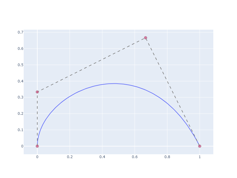

Points approximation

# Create points
import requests

foil_name = 'e1098'
url = f"http://airfoiltools.com/airfoil/seligdatfile?airfoil={foil_name}-il"

response = requests.get(url)
lines = response.text.split("\n")
lines .pop(0)
lines .pop(-1)

points = [ list(map(float, line.split())) for line in lines]
# Create an approximation of degree 3
from pygbs import core
from pygbs import interpolate

curve = interpolate.approx(
    points,
    deg=3
)

The green dots are representing the foil's points and the purple ones the control points of the approximating curve.

A closer look shows the benefit of approximation on stiff interpolation, in the case of a poorly discretized profile the algorythm is able to produce a smooth curve.