This section presents multivariate analysis pipelines that can be performed after quantification. **Exploratory routine** is designed to unveil structure in rna expression (single molecule number) and in co-localization. This analysis is based on [*Multivariate Data Analysis*](https://fr.scribd.com/document/876529227/Multivariate-Data-Analysis-Hair-Et-Al-7th-Ed-2010) by *Hair and al.*
[1. Exploratory analysis](#exploratory-analysis)
[1.1 About independent techniques](#about-indepedent-techniques)
[1.2 Rna expression analysis](#rna-expression-analysis)
[1.3 Co-localization analysis](#co-localization-analysis)
[2. Analysis parameters]
# Exploratory analysis
What I call exploratory analysis is usually refered to as indepedent techniques in multivariate analysis. They are designed to find underlying structure in data.
This pipeline focuses on **Principal component analysis (PCA)** and on **Multiple correspondence analysis (MCA)**. They are analogue techniques that identify structure in data using dimension reduction.
When looking at indepedent multivariate analysis results keep in mind that the analysis will always yield some sort of structure and should be use as exploratory results to create or investigate hypothesis **not as tools to establish causality relations.** Some indicators are computed to help you assess the relevance of the structures found.
## About indepedent techniques
Multivariate techniques are designed to unveil structural relationship between more than two variates as oposed to direct correlation analysis. To that end we different metrics can be studied (*i.e variance or mean*) through dimension reduction techniques. Dimensions (*RNA*) are grouped to explain metric (*variance*) statistic by a composition of RNA groups. The resulting groups (dimensions) contribute in a different proportion to the global metric, in the case of PCA this is materialised by their **eigenvalue**. For a sample with $N$ rna distributions we should always be able to find $N-1$ dimensions. However it does not mean that they all contribute equally to the variate, most of the time lower eigenvalues dimensions are discarded are they explain noise in the data. There are a few methods to retain an appropriate number of dimension that are detailed below in the [PCA section](#scree-plot).
Different techniques were designed to explore different aspect of the data. **PCA** technique aims at transforming correlated variables into, new, uncorrelated variables. This variables are named principal components and define dimensions that explain best data variability. PCA relies on normality asumption and on the use of metrics following a scale which makes it improper for co-localization analysis where data is categorical (even binary). **MCA** comes in as an analogue technique compatible with categorical, it is build as an extension of Correspondance Analysis but the interpretation logic of its results is similar to one of PCA results. PCA focuses on explaining data through variance the analogue, in other words it finds the structure that explain the maximum of variance; the analogue value for MCA is called **inertia**. Intertia is a measure of how much co-occurence pattern in the data deviates from independence which makes it an intuitive indicator for co-localization patterns.
The described methods below are meant to help you find or check patterns in your data using Sequential Fish built-in pipelines.
## RNA expression analysis
In this pipeline we investigate reliationship between single molecule number in cells.
### Correlation matrix
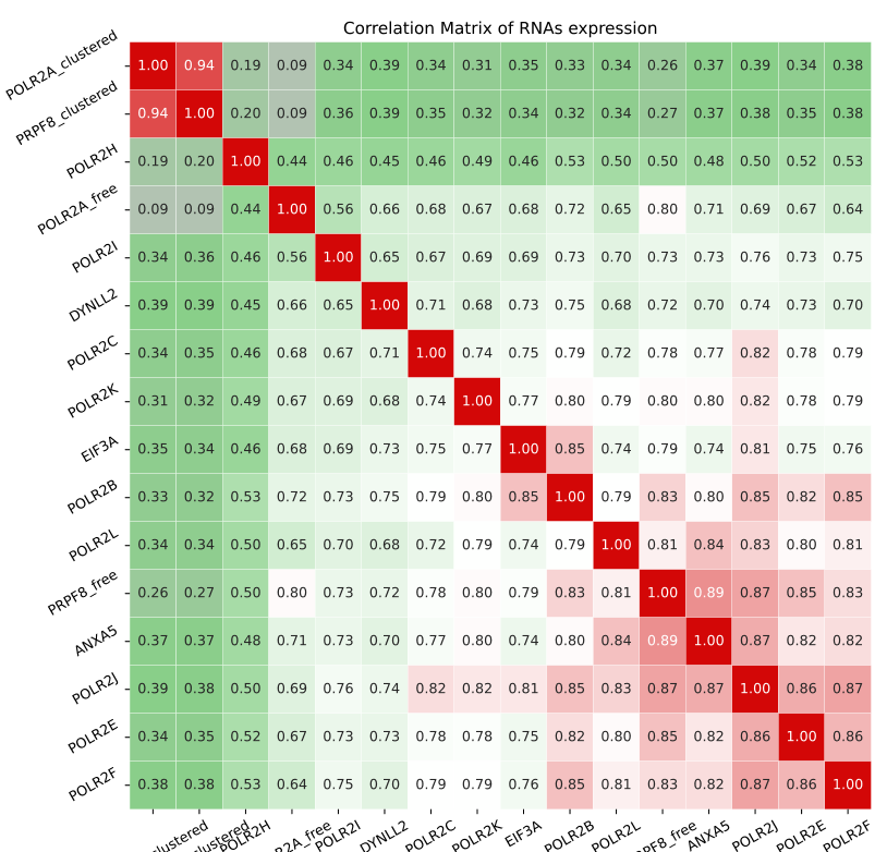
The correlation matrix is formed by computing Pearson's r coefficient to study direct correlation between RNAs. This is not multivariate analysis but it is a preliminary step to dertime if multivariate analysis is relevant. Indeed a dataset explain by direct correlation will be overly dominated by direct correlations. In such case correlated variates should be grouped beforehand or one should be eliminated to assess such as case one can refer to [partial correlations](#partial-correlation).
### Sanity metrics
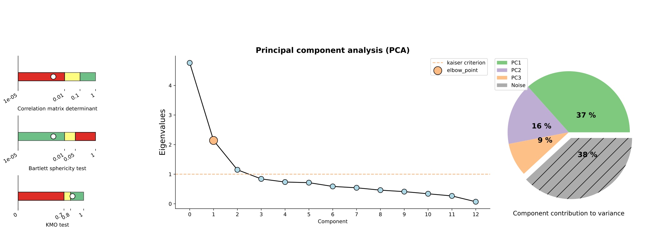
* Correlation matrix determinant : A correlation matrix determinant close to 0 (*i.e < 10^-5*) will result in mathematical instabilities when running PCA in such a case user should proceed with caution.
* Bartlett sphericity test : This indicator is a pvalue to test that correlation matrix is the identity matrix in such a case that the null hypothesis is not rejected RNAs expression are perfectly orthogonal and no underlying behavior can be found.
* Kaiser–Meyer–Olkin test (KMO) : This test sample adequacy to be interpreted throught PCA a value below 0.7 reveals critical multicolinearity within sample making dimension reduction inadequate. Sample with KMO > 0.7 are acceptable and >0.8 are interesting to investigate.
> **About the use of 'foci rnas' option**
> Using this option user can split a population in its **free** and **clustered** part. This two new population will be added to the existing population meaning that *population_A* can coexist with *population_A_clustered* and *population_A_free*. Needless to say this will create artificial correlation and colinearity in the data when running PCA make sure to remvoe your 'focis rnas' option ***or*** to filter out the main population using the **filter rna** population.
### Number of dimension
This plot aims at help you consider which dimensions are relevant for analysis and which contribute mostly to noise. There are three ways of selecting an appropriate number of dimensions for the PCA analysis. First is called **Kaiser criterion** and states that one should retain all dimensions whose eigenvalue is superior to 1. Second is to draw the eigenvalues in an ordinated manner (scree plot) and consider the elbow point of the curve as the threshold for selecting dimensions. Third is to retain as many dimensions as to explain 80% of the data variance this can be visualized in the pie plot.
During this automated analysis **we use the Kaiser criterion**.
### New dimensions and loadings
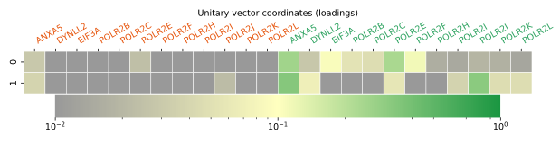
PCA yields new orthogonal dimensions explaining a part of total variance. On each of these dimensions rnas contribute differently. The contribution of an rna to a dimension is called **loadings** and is the heart of the analysis. When a group of rnas loads heavily on a dimension it means that part of the sample variance is explained better by the group than by the individuals. The ***loadings*** plot allow us to identify the principal components of the new dimensions and thus define and underlying structure of the data.
The results must be interpreted with caution and be used as guides to create or strengthen hypothesis as they are not proving cause-effects relationship, only structural behavior. What is more every data set will yield an underlying structure even if in poorly correlated data this structure will only explain **noise**.
Noise can random because your data is poorly correlated and there is no interesting underlying structure to study, or coming from biological processes that are not of interest to you (cell cycle, cell stress...) and inducing a correlated behavior to your sample. To account for biological noise we propose a few extra tools : **partial correlation** and **normalisation using control genes**.
### Partial correlation
Partial correlation isolates the **direct** linear relationship between two population. It can be used as an indicator on validity to use PCA analysis and on controlling for irrelevant biological effects. The validity of PCA analysis is already controlled using the **KMO** test, [see above](#sanity-metrics), which is based on partial correlation.
In the non-normalised figure, when partial correlation is ran, each pair uses all the other genes as covariates. Meaning we look at the direct linear relation between the pair after removing the effect of **all other population**. Obtaining very high values for a pair at this point suggest that their expression is explained **only by each other** and there are no structural effect to uncover. In such a case you can either group them (mean or median rule...) or remove one from analysis so that their correlation effect doesn't dominate the structural analyis.
In the normalised figure partial correlations is computed using control genes as covariates. In this case finding low partial correlations (**i.e < 0.3**) suggest either that your data set is poorly correlated and there is no structural effect to uncover or that the structure is dominated by noise that is captured is the control genes. In those cases normalisation using control genes is relevant. If partial correlations are strong (**i.e > 0.5**) PCA is already valid and not driven by the noise captured by the control genes, normalisation is not relevant.
## Co-localization analysis
Although this approach was initialy implemented for rna expression analysis I try to adapt it to co-localization. The pipeline is based on the ***colocalization truth table*** also computed in the [colocalization section](./analysis_colocalization) submodule. This table indicate for each spot (rows) **True** in the columns *Population_A* if the spot co-localizes with population A else **False**. The column corresponding to the spot population is always **True**. Principal component analysis requiring normal metrics, the usage of boolean data constrains to switch to **Multiple correspondence analysis (MCA)** an extension of [correspondance analysis](https://en.wikipedia.org/wiki/Correspondence_analysis) with an interpretation analogue to PCA.
### Multiple correspondence analysis
Multiple correspondence analysis (MCA) was chosen as an analogue technique of PCA for usable for boolean data. Refer to [above section](#about-indepedent-techniques) for a thorough insight. Instead of maximizing variance when reducing dimensions MCA aims at maximizing **inertia**. In this context inertia is defined as how much data deviates from complete independance.
### Scree plot and loadings
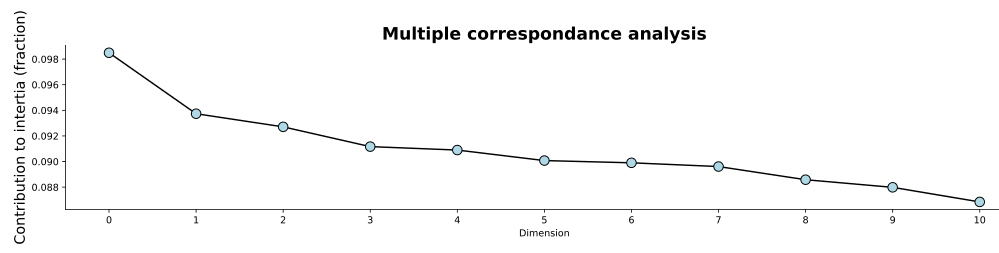
The scree plot helps you retain the best number of dimensions in your analysis. Similarly to PCA, **coordinates** x-axis is showing dimension but instead of eigenvalues, on y-axis is plotted contribution to intertia as a fraction. In MCA we usually keep dimensions contribution to more than **10%** to global inertia, one can also use the elbow point rule.
Loadings are replaced with **categories coordinates** (1 category = 1 reduced dimension) in reduced space. While we use them to understand resulting structure unveil by MCA their interpretation is quite different. Firstly, note that vectors point from origin to categories are **not unitary vectors** their squared sum equals to the inertia contribution of this dimension. What is more the scaling is done in such a way that the distance between categories reflects their dissimilarity in co-occurence patterns. In other words, **proximity between categories indicates similar co-occurence patterns** and **distance from origin indicates strengthness in contributing to intertia**. However given the number of population this can be difficult to represent on a scatter plot. To envision this information we propose the use of a heatmap indicating structure of reduced dimensions combined with a bipartite network graph.
The network graph is composed of two types of nodes :
* **Rnas nodes** *round* : Size is proportionate to rna abundancy, their are linked to a category node if they contribute to more than 2% (threshold can be modfied in parameters) to global inertia through a reduced dimension. The edge sizes are proportionate to coordinate value.
* **Categories nodes** *diamond* : Size is proportionate to contribution to global inertia. They are fully connected to each other through a weighted edge representing their proximity, more precisely, chi-squared distance is used (natural metric of MCA).
The network is display in a spring-force layout allowing similar categories to be close and dissimilar categories to be far away.
### Hierachical Clustering
Then final indicator of this multivariate pipeline is based on **hierarchical clustering** which is a **clustering** technique. Controray to MCA, that looks for structure or patterns of co-occurence this will focus on actual co-localization frequencies **ignoring underlying structure**. This **sequentialy group pairs of rna that have a high number of co-localization events** this will favorise highly expressed populations if they show co-localization. Is more meant to identify groups of rnas that have the potential of making a significant biological interaction rather than looking for group of rnas that are driven by a similar effect to co-localize. Hierarchical clustering can be interpreted as a sort of ranking of colocalizations event and is represented trought a **dendogram**. The sequentialy mechanic of this clustering will merge groups in an order based on their similarity (co-localization frequencies) and ends up by forming a group containing all rnas. The similarity between groups (x-axis) is computed using the **Jaccard distance**.
# Analysis parameters
**Control genes** (list) : List of names that were imaged as control genes in your experiment. This allow the creation of the normalised figure for the [rna expression analysis](#rna-expression-analysis).