This Python Dashboard is about Olympic Games, it summarizes more than 100 years of Olympic Games and highlight some specific performances and statistics.
The Dashboard is built with Python3 and Dash, graphs are powered by Plotly:
The Olympics Games Datasets:
The Python's depencies required for the compilation are :
- Dash : https://dash.plotly.com/installation
- Pandas : https://pandas.pydata.org/docs/getting_started/install.html
- Plotly : https://plotly.com/python/getting-started/#installation
- Numpy : https://numpy.org/install/
- Scipy : https://scipy.org/install/
Once you have installed Dash and all others dependecies, you only need download the code and execute the main python file (python main.py). All the datasets are already included, but can still be retrieved online:
- athlete_events.csv : https://www.kaggle.com/heesoo37/olympic-history-data-a-thorough-analysis
- athletics_results.csv, running_results.csv, swimming_results.csv : Via the file scrap.py (website : https://olympics.com/en/olympic-games)
When the code is executed a localhost link appears, you need to click on it, it will show the Dashboard on a website.
Usually the link is http://127.0.0.1:8050/.

We will try to summarize the dynamics behind these analytics.
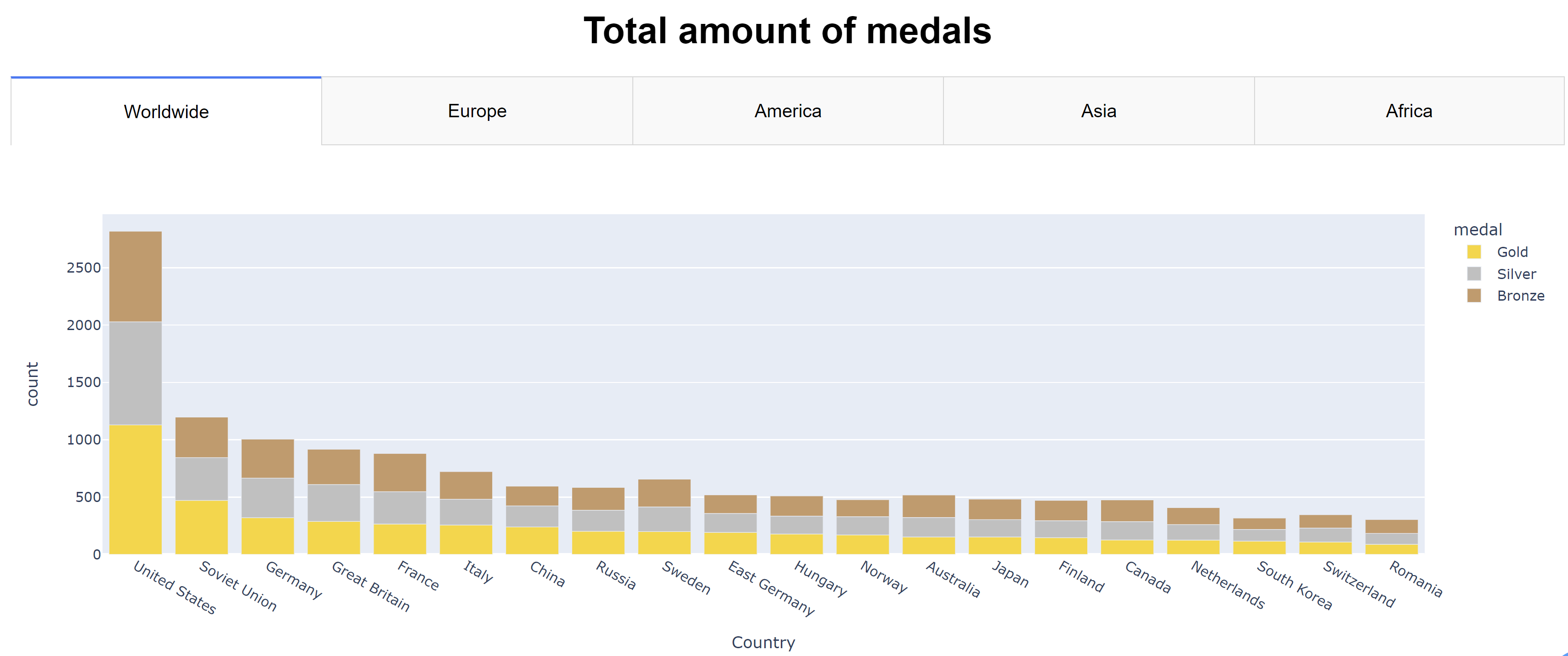
Here we can see that United States are the strongest nation in the Olympic Games, they are folowed by the Soviet Union which no longer exist since 30 years, it does mean that during their 68 years of existence they were enough dominant to not be outdated. Further there is East Germany which is in almost in the same case. Overall we see that Western countries are the strongest even if China, Japan and South Korea are well positionned.
| America | Asia |
|---|---|
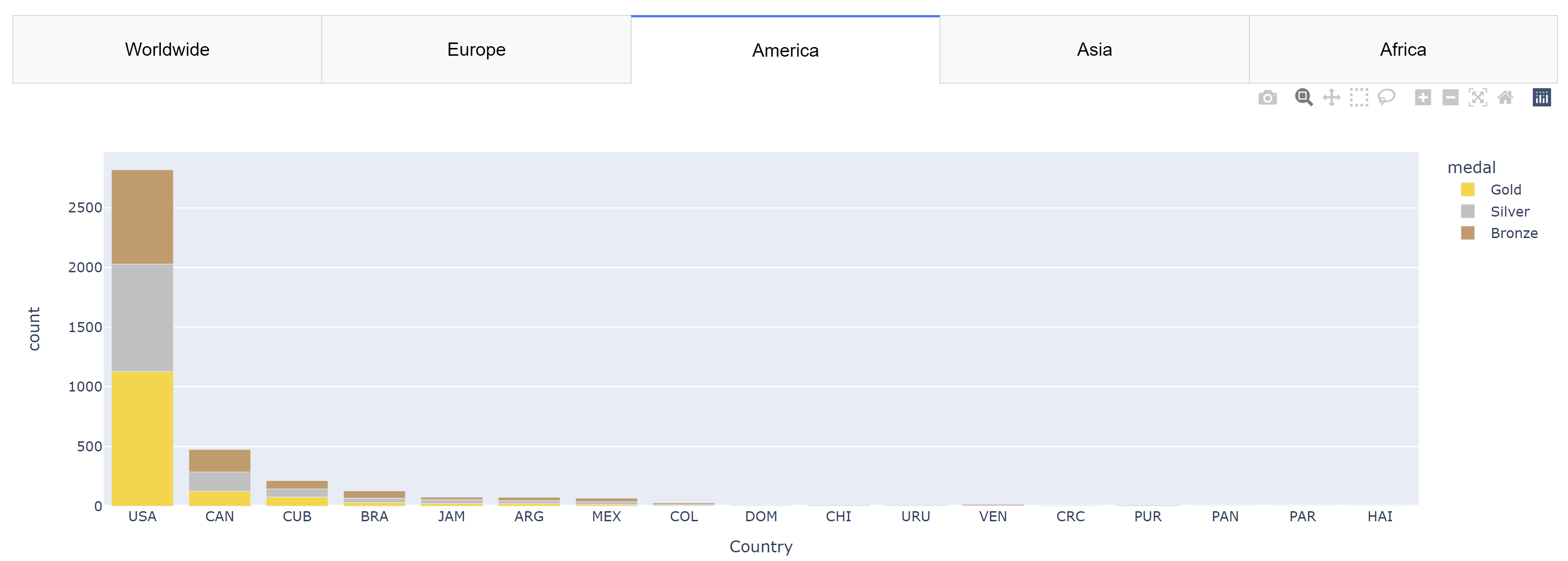 |
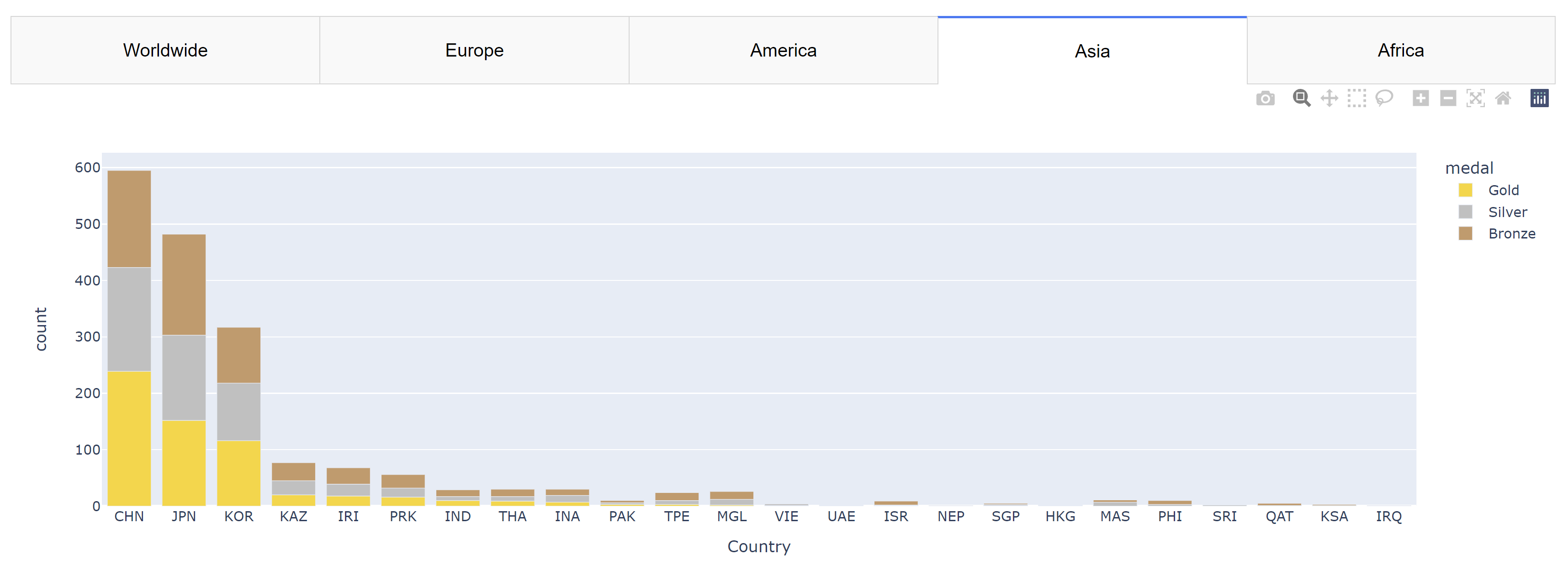 |
It clearly shows American, Korean, Japanese and Chinese dominance in their respective regions.
| 1936 | 2016 |
|---|---|
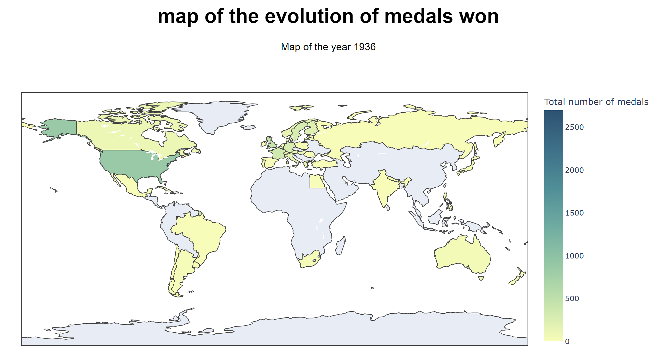 |
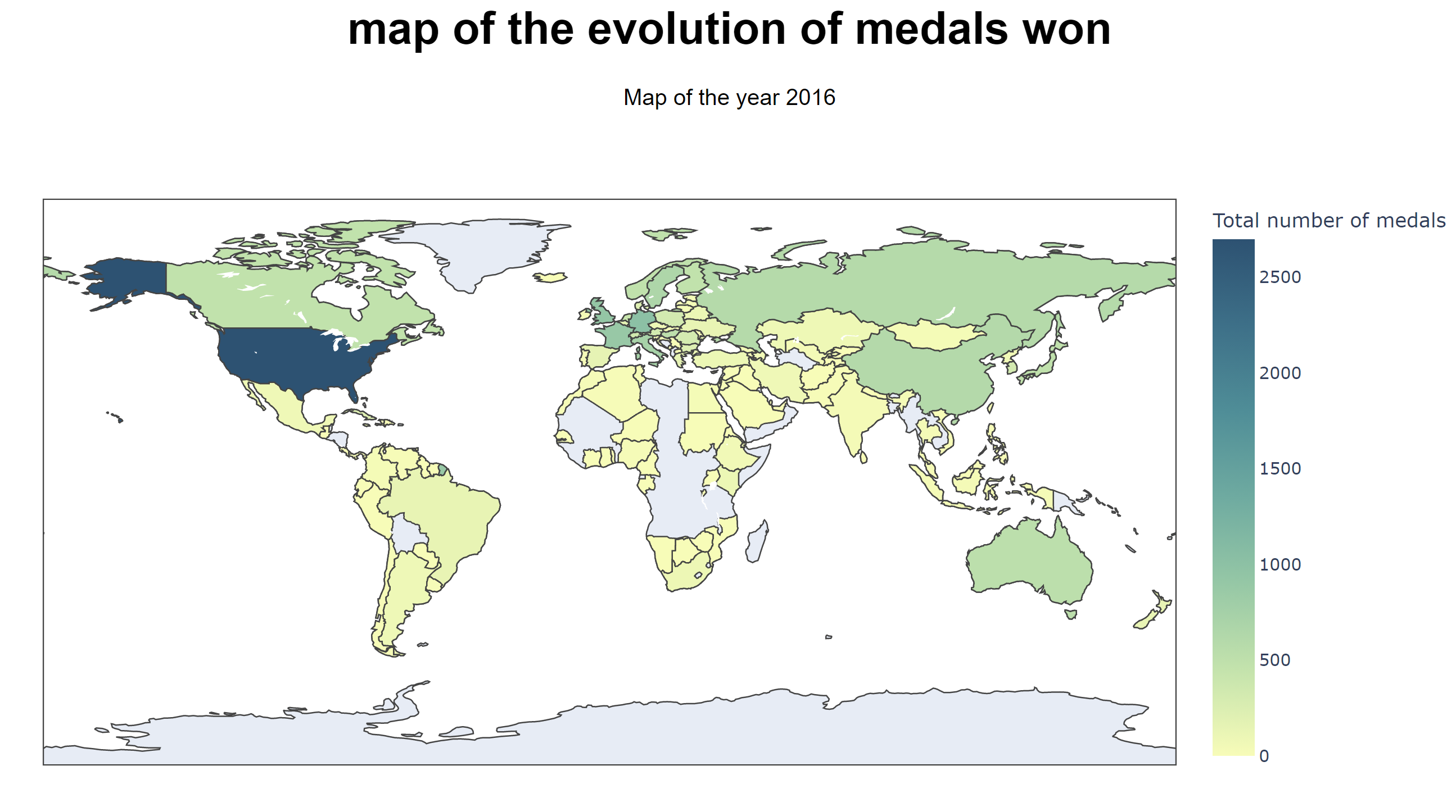 |
This Map is about the evolution, so it's better to see it scroll in the app. But what we can say is that United states has been first since the beginning and that some countries has never gained any medals and some others has obtained their first ever medal quite recently.
| Athletics | Gymnatiscs |
|---|---|
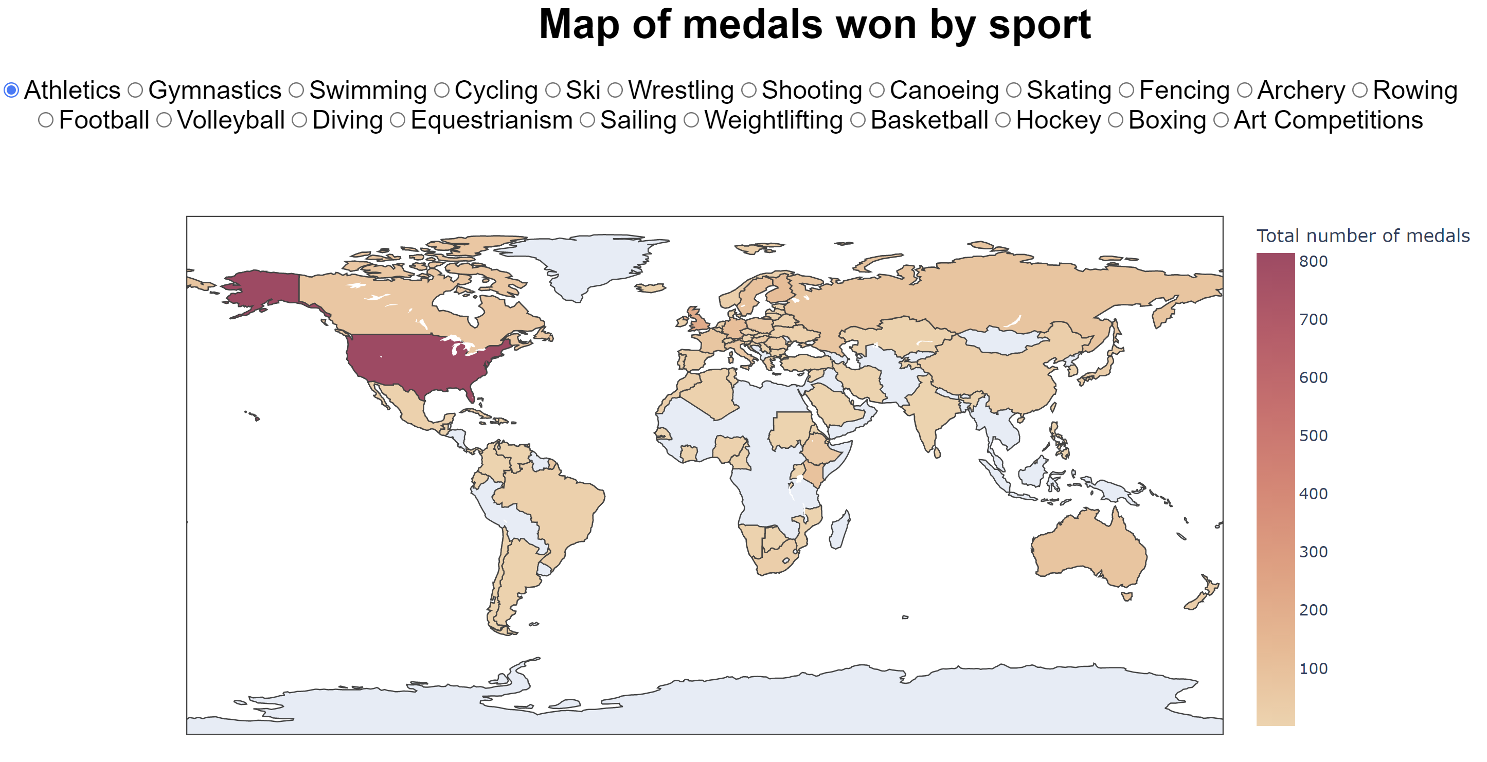 |
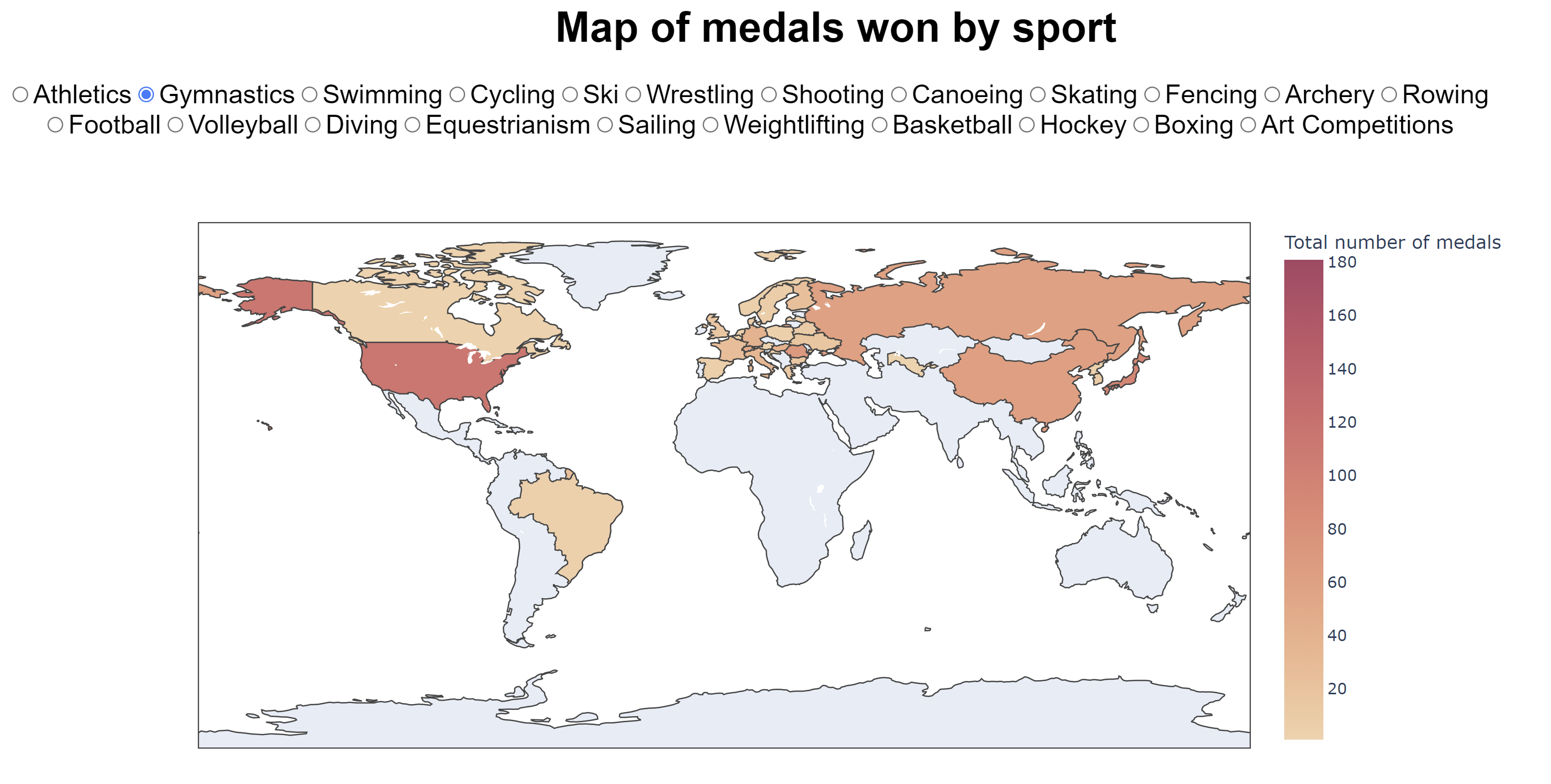 |
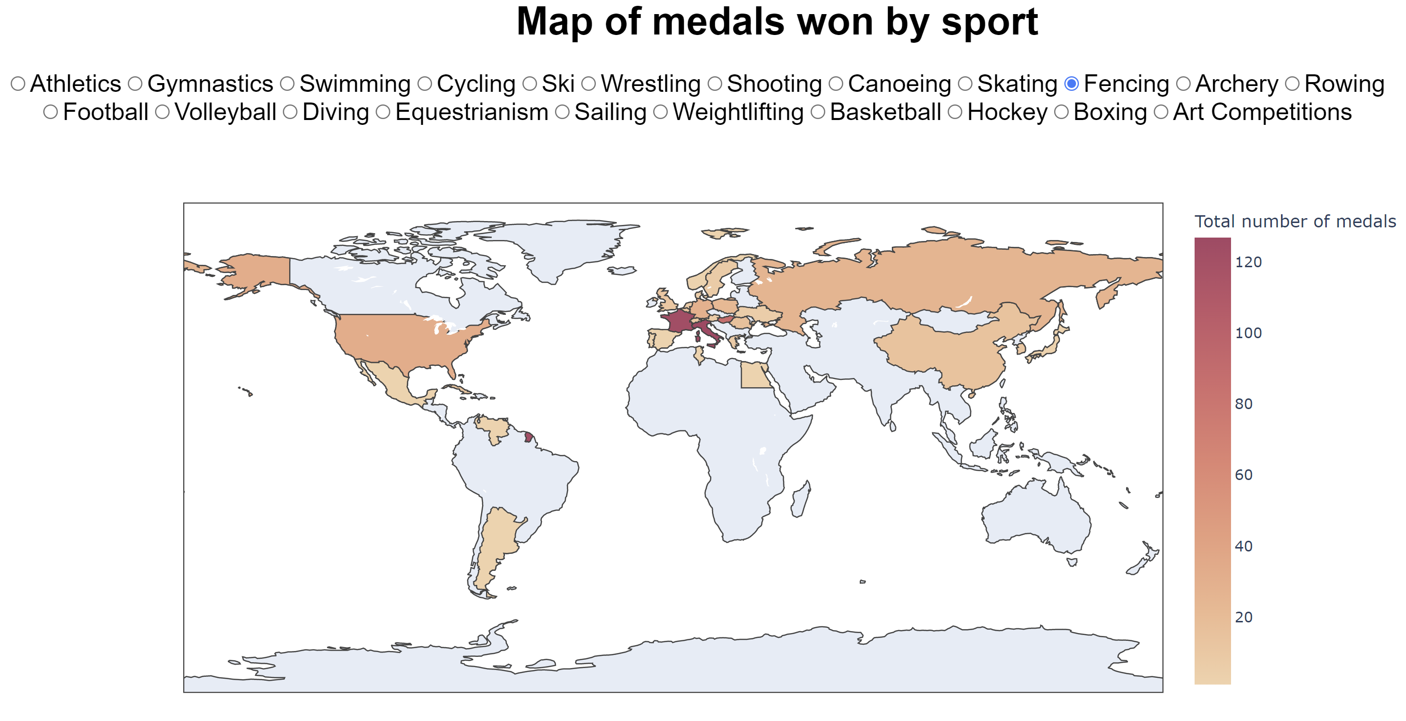
| Skiing | Fencing |
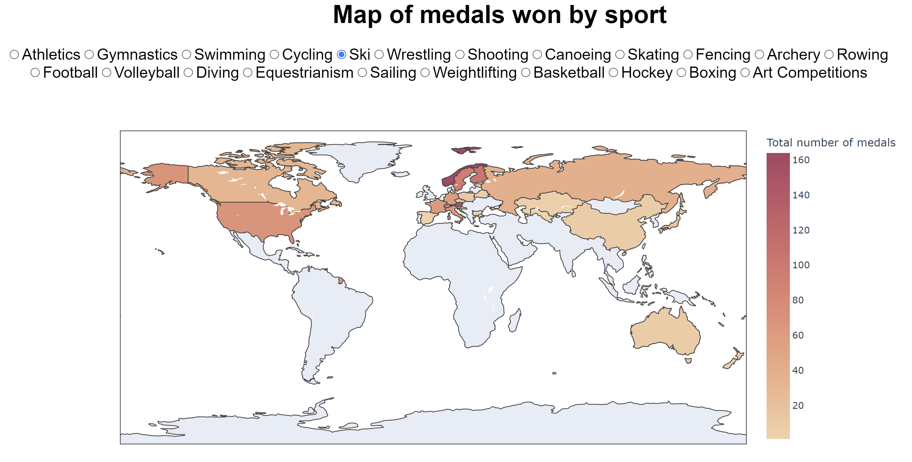 |
 |
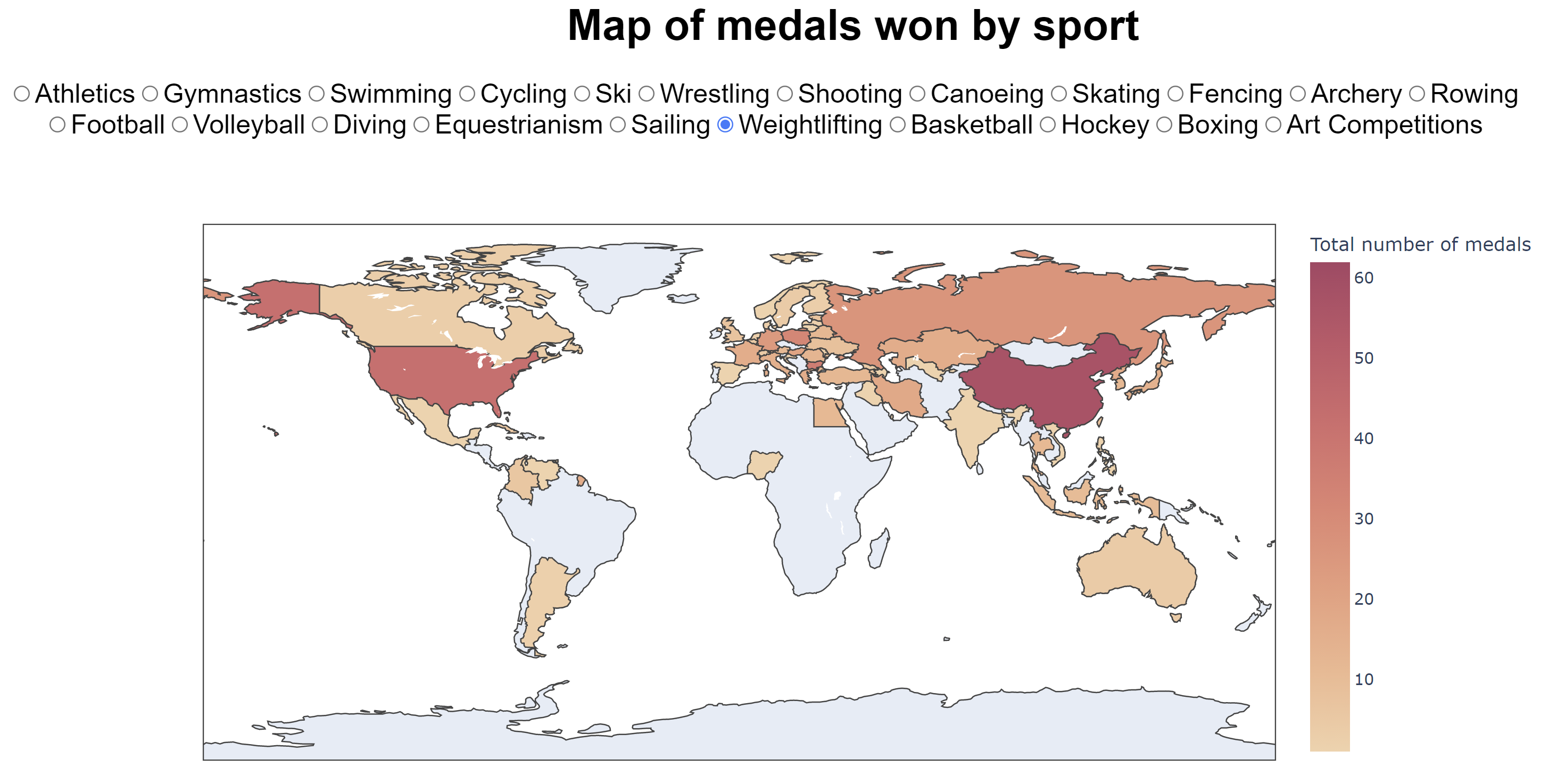
| Weightlifting | Conoeing |
 |
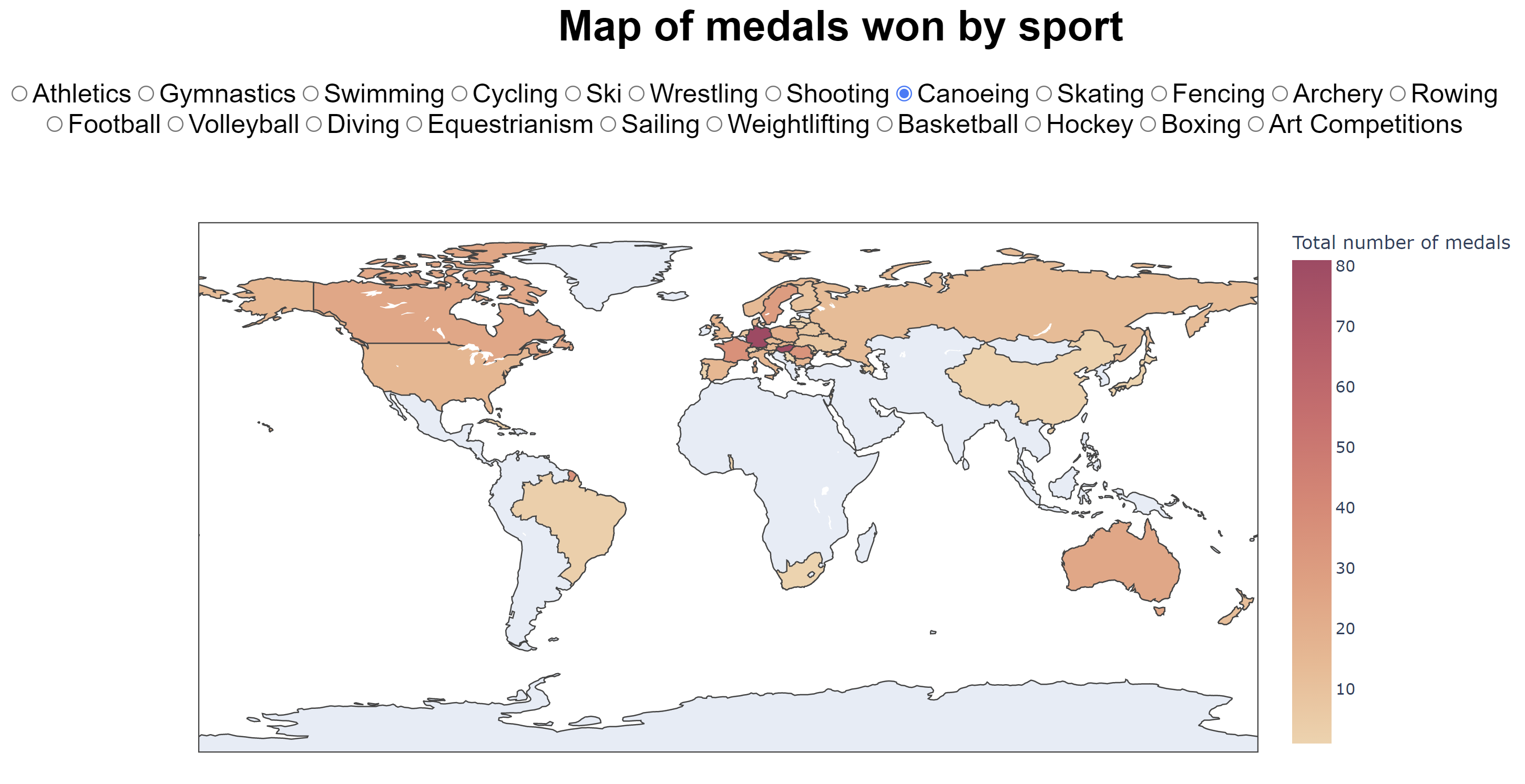 |
These maps shows that the U.S are strong on almost every sport, it also shows that some countries have their favourite sports like France and Italy with fencing and Germany with canoeing. The Gymnastics and Weightlifting maps present a great confrontation between the U.S and China and the skiing map confirms that the Nordic countries are the strongest on skis
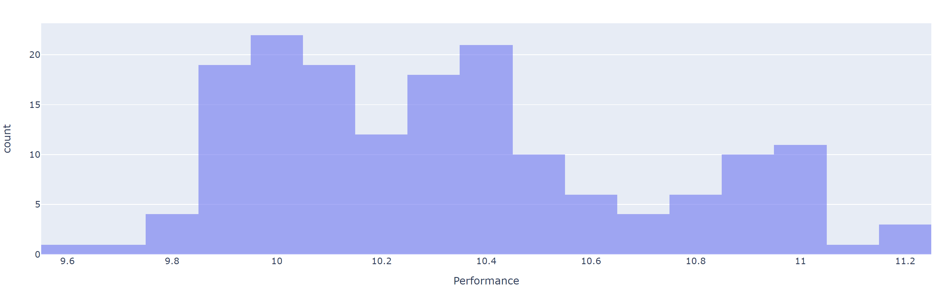
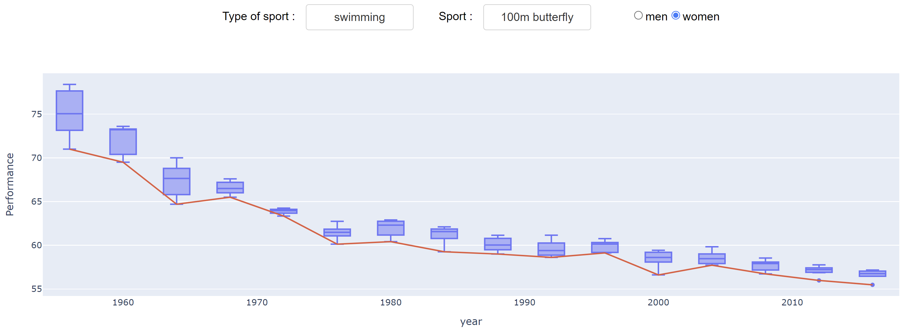
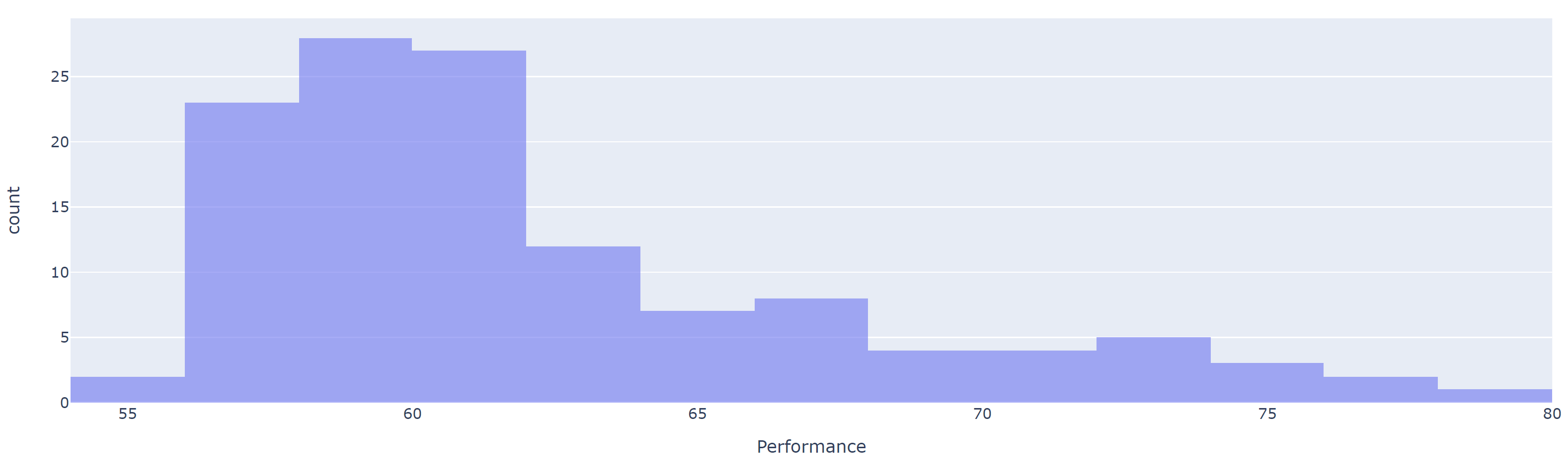
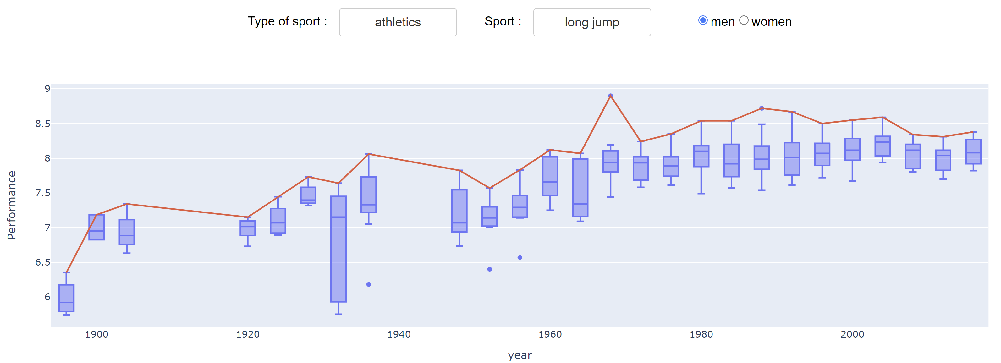
| Boxplot | Histogram |
|---|---|
 |
 |
 |
 |
 |
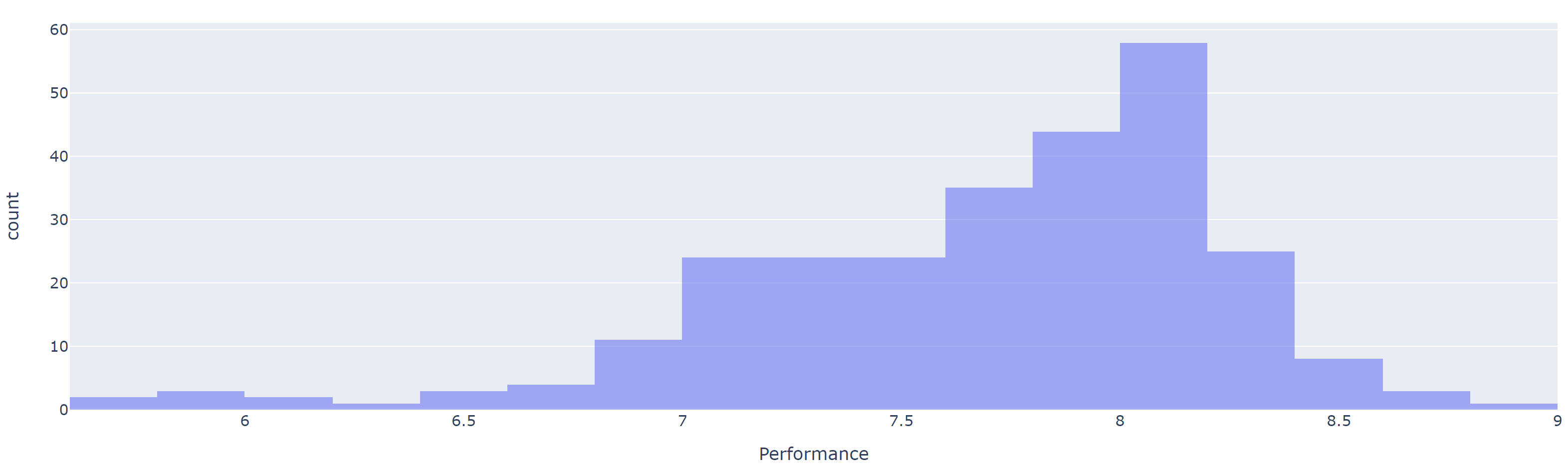 |
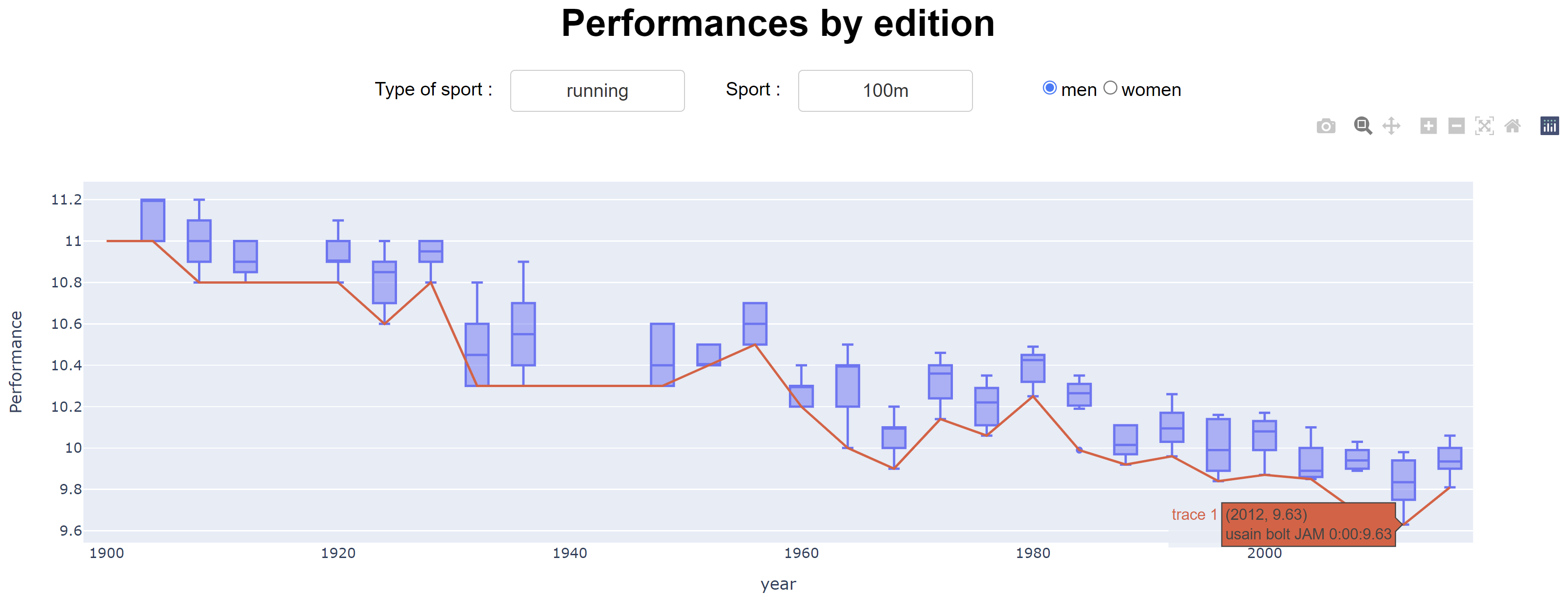
What is most striking is that the athletes have progressed a lot since the beginning of the Olympics. In all the fields, the performances improve with time before stabilizing a little, in general since the years 70-80. Therefore, we can expect that worlds record become rarers and that athletes reach a point where the human body can't go further. The Histograms highlight that 'good' performances are common because most of the results are not so far away from the record but doing a truly great performance is very rare, combined with the fact that boxes in the boxplots are getting smaller and smaller we can conclude that the athletes performances are increasingly close and good.

Here we have the height and weight displayed by sport and gender. We observe that there are notable differences depending on the sport. We already observe a certain trend between the Weight/Height ratio but some sports are totally out of this trend. Indeed if we take the case of men, we see that gymnasts meet this trend, but they are the smallest, as well as the lightest. Conversely, we have sports like volleyball or basketball where men are the tallest and among the heaviest. Among those who do not follow this trend, we find for example the Weightlifters who have to be very heavy and small. Or tug-of-war athletes who must be as heavy as possible. This is not surprising, as we can see that each sport requires very specific characteristics of size and weight depending on the type of sport, power or agility, team or individual, combat or precision etc.
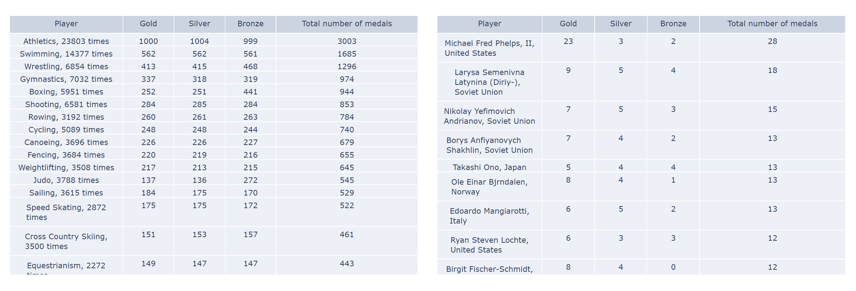
These tables summarizes who won the most medals and which sport give the most medals, we can see that sport that most people will think about when thinking about olympics games are indeed the most represented. The second table shows for instance how Micheal Phelps is a legend of the olympics and that he has a very impressive number of gold medals compared to the others, we also see that a lot of athletes played for the Soviet Union which demonstrate their power at the time. Nevertheless there is a majority of American athletes in the first places of this list.

GDP and Population values are log values, so the real distibution is wider. We see that there is kind of a threshhold to be a succesfull nation in the olympic game, nations with a not enough aumount of GDP and population all have less than 30 medals. We also can see that the medals are more correlateed with GDP than population.
We can see the history of sports at the Olympic Games since their creation. The first Tab contains all the sports and all the editions, with so much information, it is difficult to visualize well, so the other Tabs allow to restrict them in 4 categories: The sports that have always been there (first editions until today), in summer then in winter The sports that are not represented since 1950 and the sports that appeared after 1950 and are still present.
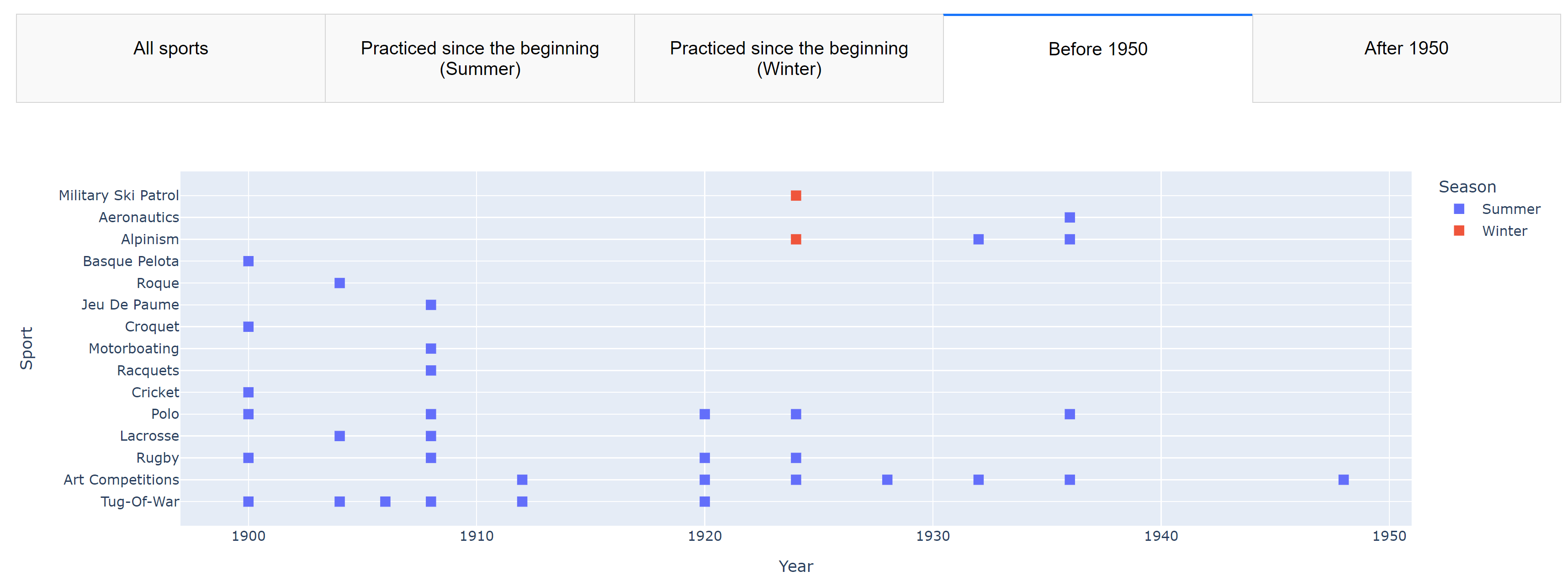
This scatter plot traces the history of sports at the Olympic Games, here you can see old sports that have long since disappeared. For example, there was once an edition with a military ski patrol, there were also sports a little more fun like Tug-of-war, Basque pelota, Jeu de Paume etc. Or some more specials categories like Alpinism or Aeronautics which rewarded exploits made in these fields.
 We can also notice that sports such as ice hockey and figure skating were present during summer games before the creation of winter games in 1924.
The code is composed of three major parts which we will explain
Our study is based on a database "120 years of Olympic history: athletes and results" available on Kaggle: https://www.kaggle.com/heesoo37/120-years-of-olympic-history-athletes-and-results It contains 271116 data on all the editions of the summer and winter Olympic games since 1896, that is 51 editions. It provides us the following information:
| Name | Information | Type |
|---|---|---|
| ID | Unique number for each athlete | Integer |
| Name | Athlete’s name | String |
| Sex | Athlete’s gender | Char (F or M) |
| Age | Athlete’s age | Integer |
| Height | Athlete’s height (in centimeters) | Integer |
| Weight | Athlete’s weight (in kilograms) | Integer |
| Team | Athlete’s team name | String |
| NOC | National Olympic Committee 3-letter code | String |
| Games | Year and Season | String |
| Year | Year of the Olympic Game edition | Integer |
| Season | Summer or Winter | String |
| City | City which hosted the Olympic Game | String |
| Sport | The category of the event (Swimming, Athletics…) | String |
| Event | The event (100m, marathon …) | String |
| Medal | Gold, Silver, Bronze or NA | String |
To complete this data, we have created a scraper to get the data from the official website of the Olympic games: https://olympics.com/
First we list all the editions we want to scrape, then the sports. With these two lists we generate the links of the pages to analyze in this way https://olympics.com/en/olympic-games/[edition]/results/[category]/[sport] For example for the edition in Rio in 2016 for the 100m men in the athletics category: https://olympics.com/en/olympic-games/rio-2016/results/athletics/100m-men After getting the HTML data of the page using the urllib library (https://docs.python.org/fr/3/library/urllib.request.html#module-urllib.request). we use HTMLParser from the html library - HyperText Markup Language support (https://docs.python.org/3/library/html.html). We can start to look for the important data by launching the function MyHTMLParser.scan(self, data, game_info, sport_info) by passing to it in arguments the information on the sport being studied. With this information the function will generate "info" which contains : [ The gender (M or W) , The sport , The country, the year ].
The parser will scan the page, look for a tag whose id is "event-result-row" with handle_starttag, retrieve the following data with handle_data. Once the important data is retrieved, we use save_row to add information about the rank, the name, the country and the result. If the result is a time, we format it to follow this pattern : 0:00:00.00 . For example 9s58 will become 0:00:09.58. We also merge this information with the information of the event stored in infos to have in the end : [gender, sport, location, year, rank, name, country, results] that we add to all the other scraped data. We repeat the operation for each "event-result-row" tag, then for each sport in the list, then for each edition of the games. For simplicity, a Sport class has been created to contain the information about the sports categories studied in our work. (running, athletics and swimming). You have to modify sportSelected to choose the desired sports. Once all the data is scraped, we write it all in a csv file.
we decare locals variables like conversion tables and NOC codes.
Then, as you can see below, we read the csv files, take infos that we want and reformart the datas into a dataframe.
 We do that multiple times and each time, depending on the finale graph that we want, the csv file, the selected columns and the format are different.
Sometime we have to write a function to do theses steps in a more personnalized way, the function will be called later.
We do that multiple times and each time, depending on the finale graph that we want, the csv file, the selected columns and the format are different.
Sometime we have to write a function to do theses steps in a more personnalized way, the function will be called later.
There we define the architecture of the application with HTML elements, Dash core components and graphs.
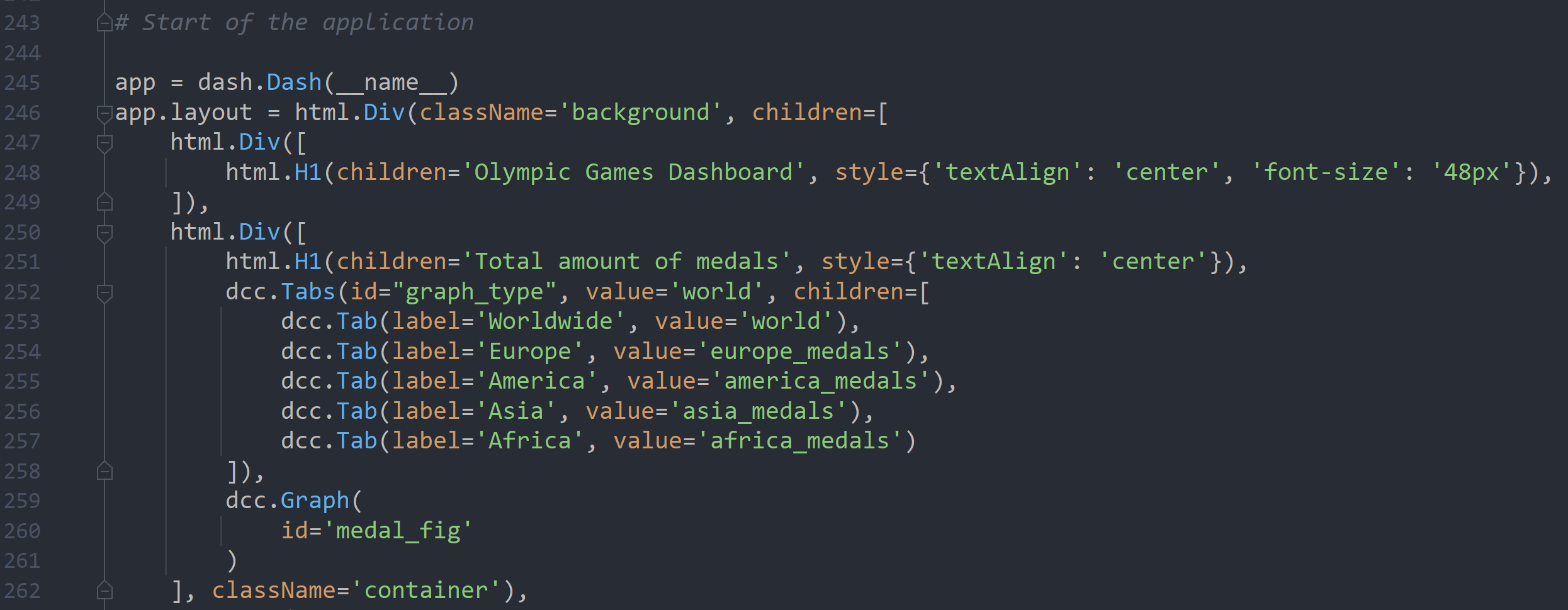 It is designed as classic HTML files, but the main elements are premade Dash Core Components (dcc) and plotly for the graphs.
https://dash.plotly.com/dash-core-components
All the graphs are in the dcc.Graph() component.
The optionals choices are made by component like dcc.Dropdown(), dcc.RadioItems(), dcc.Slider(), dcc.Tab()...
It is designed as classic HTML files, but the main elements are premade Dash Core Components (dcc) and plotly for the graphs.
https://dash.plotly.com/dash-core-components
All the graphs are in the dcc.Graph() component.
The optionals choices are made by component like dcc.Dropdown(), dcc.RadioItems(), dcc.Slider(), dcc.Tab()...
We also have to customize some styles there and use classnames which are written in assets/typographie.css.
To summarize, to add a basic component, you need to add a dcc.Graph() component containing the plotly figure or, if you want to make it interactive. Give it an id that will be used as an output in a callback function:
The screen below is a basic callback, we use elements' ID to interact with them as output/input.
 We link inputs/outputs with a function to return a graph or to update some elements.
A callback is called when an event occurs on one of its inputs. This can be a different choice in a dropdown for instance.
What is returned will replace/update the component set as output.
We link inputs/outputs with a function to return a graph or to update some elements.
A callback is called when an event occurs on one of its inputs. This can be a different choice in a dropdown for instance.
What is returned will replace/update the component set as output.
The scrap.py file has been used to generate Running_results, Swimming_results and Athletics_results csv files. This file is now useless but can be upgraded to generate new datas. The asset folder contains the styling css file and the app's icon.