data_model

Research notes Felix A Kruger

email: fkrueger@ebi.ac.uk This document was compiled using knitr:

library(knitr)
knit('data_model.Rmd')

read_chunk("../summaryPlots_bw.R")

Data loading and filtering.

library(ggplot2)
theme_set(theme_bw())
sample_infile <- "../data/sampledFrame.tab"
para_infile <- "../data/paralogs_chembl_10_compara_62.tab"
ortho_infile <- "../data/orthologs_chembl_10_compara_62.tab"

# Loading.
load <- function(infile) {
    input_table <- read.table(infile, sep = "\t", header = TRUE, na.strings = "None")
    data <- as.data.frame(input_table)
    return(data)
}

orthoFrame <- load(ortho_infile)
paraFrame <- load(para_infile)
sampleFrame <- load(sample_infile)

# Filtering.
filter <- function(data) {
    data$diff <- data$afnty1 - data$afnty2
    data <- data[abs(data$diff) < 20 & data$diff != 0, ]
    return(data)
}

orthoFrame <- filter(orthoFrame)
paraFrame <- filter(paraFrame)
sampleFrame <- filter(sampleFrame)

Fitting Laplace functions.

# Analogous Models.
require(lawstat)
require(fitdistr)
ana_laplace <- function(data) {
    scale <- mad(data$diff)
    location = median(orthoFrame$diff)
    laplace <- dlaplace(data$diff, location = location, scale = scale)
    return(laplace)
}

ana_normal <- function(data) {
    scale <- sd(data$diff)
    location = mean(orthoFrame$diff)
    normal <- dnorm(data$diff, mean = location, sd = scale)
    return(normal)
}

ortho_laplace <- ana_laplace(orthoFrame)
para_laplace <- ana_laplace(paraFrame)
sample_laplace <- ana_laplace(sampleFrame)

ortho_normal <- ana_normal(orthoFrame)
para_normal <- ana_normal(paraFrame)
sample_normal <- ana_normal(sampleFrame)

# Plotting models on top of histograms.

model_plot <- function(data, normal, laplace)
{  
   data$normal <- normal
   data$laplace <- laplace
   ggplot(data) + 
   geom_histogram(aes(diff, y= ..density..), fill = "darkgrey", col = "black", binwidth = .4) +
   coord_cartesian(xlim = c(-5, 5), ylim = c(0,.7)) +
   scale_x_continuous(breaks = c(-4,-2,0,2,4))+
   geom_line(aes(x = diff,y = normal), size = .5, col = "#003366")+ #003366
   geom_line(aes(x = diff,y = laplace), size = .5, col = "#993333")
}

model_plot(sampleFrame, sample_normal, sample_laplace)
model_plot(orthoFrame, ortho_normal, ortho_laplace)
model_plot(paraFrame, para_normal, para_laplace)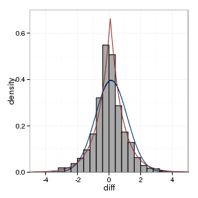

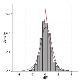
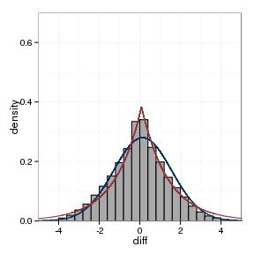
plot of chunk models

The fitted parameters are summarised below:

data set	location, laplace	scale, Laplace	location, Normal	scale, Normal
between assays	-0.006	0.752	0.0044	1.006
orthologs	0.0822	0.7679	0.1387	0.8636
paralogs	-0.0103	1.304	-0.0207	1.4254

q-q plots.

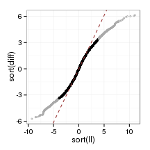
library(lawstat)
plot_qq <- function(data)
{
    data$trim <- with(data, cut(diff, breaks=quantile(diff, probs=c(0,1,99,100)/100), labels = c('trim','ok','trim'), include.lowest=TRUE))
    data$ll <- rlaplace(length(data$diff))
    x <- qlaplace(c(.18,.82))
    y <- quantile(data$diff, c(0.18, 0.82))
    slp <- diff(y)/diff(x)
    incp <- mean(data$diff)
    ggplot(data)+
       geom_point(aes(y=sort(diff),x=sort(ll), col = sort(trim)),shape  =1, size =1)+
      geom_abline(slope = slp, lty = 2, col = '#993333', size =.5, intercept = incp)+
       theme(legend.position = 'None')+
       scale_colour_manual(values = c('darkgrey', 'black'))
}

plot_qq(sampleFrame)
plot_qq(orthoFrame)
plot_qq(paraFrame)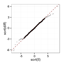

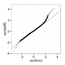
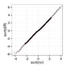
plot of chunk unnamed-chunk-5

plot_qq <- function(data){    
    data$trim <- with(data, cut(diff, breaks=quantile(diff, probs=c(0,1,99,100)/100), labels = c('trim','ok','trim'), include.lowest=TRUE))
    data$nn <- rnorm(data$diff)
    x <- qnorm(c(.2,.8))
    y <- quantile(data$diff, c(0.18, 0.82))
    slp <- diff(y)/diff(x)
    incp <- mean(data$diff)
    ggplot(data)+
       geom_point(aes(y=sort(diff),x=sort(nn), col = sort(trim)), shape = 1, size =1)+
       geom_abline(slope = slp, lty = 2, col = '#993333', size =.5)+
       scale_x_continuous(breaks = c(-8,-6,-4,-2,0,2,4,6,8))+
       scale_y_continuous(breaks = c(8,-6,-4,-2,0,2,4,6,8))+
       theme(legend.position = 'None')+
       scale_colour_manual(values = c('darkgrey', 'black'))
}

plot_qq(sampleFrame)
plot_qq(orthoFrame)
plot_qq(paraFrame)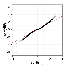

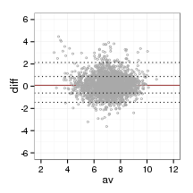
plot of chunk unnamed-chunk-6

Bland Altman plots.

bland_plot <- function(data, probs, al)
{
   data$av <- (data$afnty1 + data$afnty2)/2
   ggplot(data)+
   geom_hline(yintercept = quantile(data$diff, prob = probs[3]), col = '#993333')+
   geom_point(aes(x=av, y = diff), col = 'darkgrey', shape =1, size =1, alpha = al)+
   #geom_point(aes(x=av, y = abs(diff)-8), col = 'black', shape = 1, size =1)+
   geom_hline(yintercept = quantile(data$diff, prob = probs[c(2,4)]), lty = 'dotted', col = 'black')+
   geom_hline(yintercept = quantile(data$diff, prob = probs[c(1,5)]), lty = 'dotted', col = 'black')+
   scale_y_continuous(breaks = c(-6,-4,-2,0,2,4,6),limits = c(-6,6))+
   scale_x_continuous(breaks = c(0,2,4,6,8,10,12),limits = c(2,12))
}

probs <- c(2.3, 15.9, 50, 84.1, 97.7)/100
bland_plot(sampleFrame, probs, 1)
bland_plot(orthoFrame, probs, 1)
bland_plot(paraFrame, probs, 1)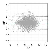

plot of chunk unnamed-chunk-7

Distribution quantiles.

library(boot)
get_q <- function(data, d, probs) {
    return(quantile(data[d], prob = probs))
}

boot_quant <- function(data, probs, R) {
    return(boot(data, get_q, probs = probs, R = R))
}

The quantiles that would correspond to one and two standard deviations of a normal distribution (2.3%, 15.9%, 50%, 84.1%, 97.7%) are the following for the inter-assay data:

boot_quant(sampleFrame$diff, probs, 1000)

## 
## ORDINARY NONPARAMETRIC BOOTSTRAP
## 
## 
## Call:
## boot(data = data, statistic = get_q, R = R, probs = probs)
## 
## 
## Bootstrap Statistics :
##      original     bias    std. error
## t1* -2.202687  0.0089816    0.081512
## t2* -0.810184 -0.0027613    0.033331
## t3* -0.006012 -0.0005573    0.008542
## t4*  0.875835  0.0010595    0.028695
## t5*  2.136645  0.0123701    0.086393

The quantiles that would correspond to one and two standard deviations of a normal distribution (2.3%, 15.9%,50%, 84.1%, 97.7%) are the following for the ortholog data:

boot_quant(orthoFrame$diff, probs, 1000)

## 
## ORDINARY NONPARAMETRIC BOOTSTRAP
## 
## 
## Call:
## boot(data = data, statistic = get_q, R = R, probs = probs)
## 
## 
## Bootstrap Statistics :
##     original     bias    std. error
## t1* -1.45284 -0.0091009     0.04732
## t2* -0.61904 -0.0003034     0.02310
## t3*  0.08219 -0.0007194     0.02010
## t4*  0.87506  0.0027265     0.01954
## t5*  2.13212  0.0076835     0.12577

The quantiles that would correspond to one and two standard deviations of a normal distribution (2.3%, 15.9%,50%, 84.1%, 97.7%) are the following for the paralog data:

boot_quant(paraFrame$diff, probs, 1000)

## 
## ORDINARY NONPARAMETRIC BOOTSTRAP
## 
## 
## Call:
## boot(data = data, statistic = get_q, R = R, probs = probs)
## 
## 
## Bootstrap Statistics :
##     original     bias    std. error
## t1* -2.94803  0.0018315     0.01704
## t2* -1.41933  0.0009791     0.01224
## t3* -0.01032  0.0009237     0.00795
## t4*  1.34714 -0.0005763     0.01275
## t5*  2.92636 -0.0014636     0.02437

Provide feedback

Saved searches