VEX for artists

Introduction

For those who tried or even afraid to begin to learn VEX but fail and stop because it was too hard.

Here you will learn VEX and applied math starting from the basics. From general to specific, keeping things extremely simple, with a detailed explanation we will go through the process of solving problems with the help of programming.

In order to follow you need elementary knowledge of Houdini UI and an essential understanding of core programming concepts. If you can render the metal sphere and able to distinguish a loop form variable, then you are fine to go. If not, that is also fine. Check Programming Basics tutorial if you are a total noob in developing.

The only important thing you really need to start is a strong desire to finally kick off the VEX code by yourself, not just copying symbols from arbitrary tutorials.

This article is structured in a way that the beginner information locate on top and the more you go down, the more advanced it becomes.

Article content:

• VEX orientation
  Attribute Wrangle | Point concept | Create point | Create line | Create circle
• VEX first steps
  Explore functions | Sine | Noise | Repetitive patterns
• Solving problems with VEX
  Hanging a wire | Checker | Polar checker | Blur |
• Vectors
• VEX next steps

All exercises from this chapter you can find in VEX snippets hip file

VEX orientation

The goal here is to start with the straightforward and basic tasks keeping the amount of code minimal and gradually, step by step increase the complexity of exercises. If you will really understand the basics it would be easy to develop extra functionality for the staring code.

Attribute Wrangle

The Attribute Wrangle node creates or modifies existing geometry with a code written in VEX language.

Any code written in any programming language needs to be compiled (converted from human-readable form to machine code) and executed. Some languages like Python do code compilation behind the scene, so you just run the code and get results. Usually, any program takes something as input, produce some computations, and output some results.

E.g. print 2 + 2 program in Python will produce the addition + of two input values 2 and 2, and output the result of 4.

The Attribute Wrangle node is a container for the VEX code which allows making desired computation on input geometry and so you can get results from the node output.

Create a wrangle in a fresh Houdini scene

• Press TAB in Node View, type geometry, hit ENTER
• Dive inside "Geometry" node, delete "File" node
• Press TAB, type aw, hit ENTER to create the "Attribute Wrangle" node.

The Attribute Wrangle node can execute a VEX code in two different ways: serial and parallel.

Serial mode

Attribute Wrangle working in serial mode if you set the "Run Over" parameter to Detail.

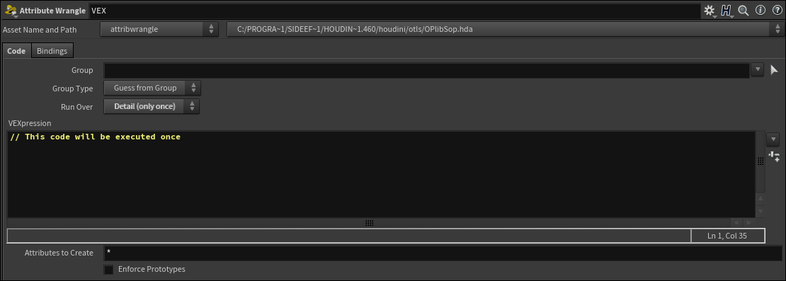
In serial mode, the VEX code written in VEXpression window will be executed once. This is the usual workflow of programming, the code executed line by line and produces some result at the end.

You don`t need to connect geometry in order to work with a Wrangle in this mode, although you can if you need it. You will be able to access your geometry attributes for every point (vertex or primitive) by their indexes.

Create Attribute Wrangle, set Run Over Detail, enter code:

printf('%s\n', 'Hello, World!');

You should have a "Hello, World!" message in the Houdini Console window. Never mind if you don't understand the code, we are just exploring the concept of code flow here.

Now connect any geometry to the first wrangle input. Let`s print the X position of the third point (index of the third point is 2):

printf('%s\n', 'Hello, World!');

vector point_position = point(0, 'P', 2);
printf('position X = %s\n', point_position.x);

In order to get a positions for all input points, you need to create an array of all those points, iterate through that array and get position for each point during each step of the iteration.

printf('%s\n', 'Hello, World!');

for(int i=0; i<npoints(0); i++){
    vector point_position = point(0, 'P', i);
    printf('ptnum %s\n', point_position.x);
}

Paralel mode

Attribute Wrangle working in parallel mode when you set the "Run Over" parameter to Primitives, Points, Vertices, or Number.

You need to have at least one point as input to be able to work in parallel mode, e.g. connect any geometry to your Attribute Wrangle. The VEX code written in VEXpression window will be executed on every point at the same time (that's why it called parallel).

It does not mean that VEX code will be executed as many times as many points you have in input, but in cases when you accessing input geometry (e.g. reading a point position) it will be done for every point at the same time.

You will be able to access your geometry attributes using build-in attributes like @ptnum, @numpt etc.

Create Attribute Wrangle, leave Run Over as Points, connect any geometry as input, enter code:

printf('%s\n', 'Hello, World!');

You should have the same "Hello, World!" message in the Houdini Console window. Nice.

Let's print the X position of the third point:

printf('%s\n', 'Hello, World!');

vector point_position = point(0, 'P', 2);
printf('position X = %s\n', point_position.x);

So far so good. What about all points positions? Here we go:

printf('%s\n', 'Hello, World!');

vector point_position = point(0, 'P', @ptnum);
printf('position X = %s\n', point_position.x);

Some parts of the code work once ("Hello, World!"), another was executed on every point. The parallel mode might be confusing even for experienced users. You need to practice a lot and you will get it.

For now, just imagine your Attribute Wrangle as a node that runs the VEX code from the VEXpression window and doing required stuff with your points.

Point concept

Point is a basement of 3 Dimensional data representation and its a core entity in Houdini. Understanding points allow understanding a huge part of SOP context (an area where you are creating models) in Houdini. To make things simple you can consider the single point as a complete geometry of any complexity.

Point in Houdini is a basic container in 3D space with a number of attributes associated with it.
Attributes are just variables on points to store data. The minimal amount of point attributes is one: point position in the scene (P). Point position is a built-in vector attribute, it holds 3 float number: point position in X, Y and Z in the global coordinate system (scene).

The attributes could be built-in (standard, already existing in Houdini) and custom (created and defined by the user). You can examine point attributes and their values in Geometry Spreadsheet window.

Attributes syntax.
You define an attribute in VEX with data type, @ sign and attribute name :

• v@myVectorAttribute;
• f@myFloatAttribute;
• i@myIntegerAttribute;

You don't need to define the data type of built-in attributes:

• Point position: @P;
• Point number: @ptnum;
• Total amount of points: @numpt;

All modeling and bunch of other operations in Houdini are just around creating and managing points and their attributes.

Create a point

Create an Attribute Wrangle, set Run Over parameter to Detail.
Now to create a point we need to know a command for that. Let`s use Google Development Technique!

Search for "create point Houdini vex" and you will definitely find out that addpoint() will allow us to solve the task. Search for "addpoint vex" to read Houdini documentation on addpoint() command.

Always start from reading the documentation for the command you wish to use, even if explanation there would not have any sense for you. This could happen at the beginning, but you will get more and more benefits from docs later, just do it to build an experience.

One of possible usage of this command is: int addpoint(int geohandle, vector pos)
What can we learn from this?

• First, this command returns point number (integer data type). Its simple, if you have 10 points, each of them will have its own index starting from 0, ending with 9. You can get access to a particular point (and point attributes) using this index. In the case with one point, we will have one point number equal zero.
• addpoint command required 2 arguments (inputs): integer "geohandle" and vector "pos". We would not go deep into geohandle concept, imagine it as a port for plugging some data and use 0 for its value, it will suit for the majority of cases. Second argument "Pos" is a vector position in 3D space, X, Y and Z coordinates of the created point.

So with addpoint() we will create a point in a given position in space.
Let's do it, write in your Attribute Wrangle node:

// Create one point at the origin
addpoind(0,0);

Turn on Display points and Display pint numbers. If you did everything right you should get one point at the origin of Houdini scene:

Check Geometry Spreadsheet to see point attributes: point number 0 has one vector attribute P which is "point position" and value of this attribute is P.x = 0.0, P.y = 0.0, P.z = 0.0

Curious minds might notice one issue: point position is a vector attribute, but we feed an integer as a second argument of addpoint() command. Despite our code works it is actually wrong, we never should mess up our data types! It's a good practice always to declare the data type explicitly. Let's also use a variable to organize our code better. Organizing one line of code may seem ridiculous but proper structuring and organization should be done to any amount of data we work with.

// Create one point at the origin
vector position = {0,0,0};
addpoint(0, position);

Where position = {0,0,0} means X, Y, Z coordinates equal 0.

Read the next section "Manage attributes" if you keen to learn more about this topic or skip the additional theory and go to the next step and create a line

Manage attributes

Ok, we create a point with a default position attribute.
Let's learn how we can create, set and get custom or built-in point attributes.

Create a new Attribute Wrangler, plug output of point creation wrangler to the first input, add a code: @N;. Check Geometry Spreadsheet to ensure that new built-in vector attribute N (normal) was added and has value {0, 0, 0}.

You can:

• initialize new attribute with value: @N = {0, 1, 0};
• set attribute value: @N = set(0,0,0);
• get attribute values: vector v@getPosition = @P; and float f@getPosition_Y = @P.y;

You can use variables (vector <variableName>) instead of attributes (@attrName). What the difference between them? You can consider variables as a local data storage within current wrangle, variable you create in one wrangle would not be visible anywhere else. Attributes a stored globally and can be accessed by downstream nodes.

If you don't need to access attribute outside the wrangle — use variables instead to keep the scene clean.

Create a line

Learning such small and easy but fundamental thing as point creation we can do a lot of powerful things! Let's do the next step and create 10 points along X-axis to build a line!

To create 10 points we need to repeat 10 times what we already learned — one point creation. Remember what programming concept we need to use in order to perform repeating? Our loop will run 10 times. Inside the loop, we will place a command to create a point:

// Create 10 points
for (int n=0; n<10; n++){
    addpoint(0, set(0, 0, 0));   
    }

Where int n=0; n<10; n++ is a description how many times we will run the code inside the loop: starting from 0, ending at 10, with a step of 1. Here n is a variable which define an iteration step: 1,2,3,4 ... 10.

Check geometry spreadsheet, we get our 10 points. Now they all share the same position {0,0,0}.

Next, we need to set a proper position for each point inside our loop to form a line. Our first point may stay at the origin {0, 0, 0} but each next point should have X coordinate increasing by the certain value — distance from the previous point: {<distanse>, 0, 0}. The most obvious and common way to define this increasing value is to use iteration step of the loop n:

// Create 10 points with 1 unit distance between them along the X-axis
for (int n=0; n<10; n++){
    addpoint(0, set(n, 0, 0));   
    }

We run through the loop 10 times and each next iteration gives us increasing by 1 point position at X coordinate (see P[x] in geometry spreadsheet). But what if we want to determine another then 1 incremental value for the X position? In other words, how we can modify the distance between points?

Since we are using iteration step value to determine coordinates we should modify this iteration step value to modify coordinates. So we will multiply the iteration step by another value, let`s call it distance coefficient. If distance coefficient would be less then 1 — the distance will decrease, and if it would be greater than 1 the distance will increase.

You should know that multiply a value by 0.5 it is the same as divide this value by 2, right? So we get increasing or decreasing of some value with the same multiplication operation. This is how we start using math to achieve our goals!

In this case, distance coefficient would be a constant (same value for each step of the loop iterations). And we can define it as a variable in our code:

// Create 10 points with 0.5 unit distance between them along the X-axis
float distCoef = 0.5;

for (int n=0; n<10; n++){
    addpoint(0, set(n*distCoef, 0, 0));   
    }

Changing distance coefficient value in the Wrangle code is not very handy and interactive. So let`s create a UI element on the Wrangle node which will drive our distance:

// Create 10 points along the X-axis
float distCoef = chf('Distance');

for (int n=0; n<10; n++){
    addpoint(0, set(n*distCoef, 0, 0));   
    }

Where chf('Distance') tells to take value from 'Distance' parameter on the Wrangle. To activate UI with this parameter you need to press a button with a slider icon right to the VEX Expression window.

There are several options for creating UI in Wrangle node:

• Integer: int integerValue = chi('Integer');
• Float: int floatValue = chf('Float');
• Vector: vector vectorValue = chv('Vector');
• Modify parameter throug ramp: float remapPosition_X = chramp('remap_P.x',@P.x);

Ok, let`s define a number of points with UI also:

// Create points along the X-axis
float distCoef = chf('Distance');
int numberOfPoints = chi('Number_Of_Points');

for (int n=0; n<numberOfPoints; n++){
    addpoint(0, set(n*distCoef, 0, 0));   
    }

To finalize line creation we need to connect our points with polygons to build an actual line.

In Houdini, to create a polygon (primitive) you need to build a primitive and add vertexes to it. To build a primitive in VEX use addprim() command, to add a vertex to a primitive use addvertex() command. We need to create one primitive and add all our points to it.

Create another Wrangle (Run Over Points) and connect points creation wrangle as a first input. Enter the code:

// Create LINE primitive
int primitive = addprim(0, 'polyline'); 
// Calculate total number of points
int numberOfPoints = @numpt;

// Create a vertex for each point in primitive
for (int n=0; n<numberOfPoints; n++){
    addvertex(0, primitive, n);  
    }

Here we create a primitive: addprim() and get a number of points we created in the first Wrangle node: numberOfPoints = @numpt, the @numpt is a built-in attribute which returns the total number of points from the first input. Then in the loop for each point we create vertex and add this ertex to a primitive: addvertex().

Create a circle

Here we come to a more fancy stuff! At this point, we will start using trigonometry to draw a circle.

In the line example we define the position of each point in 3D space using the Cartesian coordinate system by setting X, Y and Z values. This is the most intuitive and accustomed coordinate system, however not the only one. When it comes to a circle the Polar coordinate system may work better.

See the corresponding chapter in math basics section for more details.

With the Polar coordinate system, you can define point position on the plane using angle and distance from the center. If the distant would be a constant value then we can set point position on the perfect circle by specifying only the angle for each point!

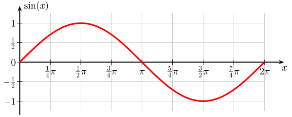
However, Houdini uses a Cartesian coordinate system to determine objects transformations (position, rotation and scale), hence you need to feed {X,Y,Z} values to addpoint() function, it would not understand the angle. So after we define point positions of the circle in Polar coordinates (angle) we would need to convert them to Cartesian (X,Y,Z). And the relationship between Polar and the Cartesian coordinate systems can be expressed through sine and cosine functions:

• position X = cosine(angle)
• position Y = sine(angle)

Very simple and elegant, right? The image from the Sine article on Wikipedia illustrates this dependency very well:

In VEX code this part will look like:

float angle = 0;
vector position = {0,0,0};
int numberOfPoints = 256;

for (int n=0; n<numberOfPoints; n++){
    position.x = cos(angle);
    position.z = sin(angle);
    addpoint(0, position);

It's time to speak about the angle. We can consider a circle as one full turn of a point around the origin. And we use to know that angle of one turn is equal to 360 degrees. Degrees (measurement of the angles) were designed for human usability and they are really good in this role, but in Math and computer graphics, you will have to deal with Radians.

Why Radians? Because radians is a mathematical angle definition based on circle attributes. One turn (360 degrees) is equal 2*Pi radians. Radians are all about the relation between circle radius and circumference:

Let`s put theory into practice an build our magic circle finally! We will use the same concept as we did with the line:

• define the number of points
• define starting angle of rotation and position
• define a segment rotation angle for each point
• in the loop (for each of point number):
  • create a point
  • set point X and Y coordinates through the angle
  • increment angle by segment rotation angle

The number of points could be either constant (12 points) or user-defined with UI variable:
int numberOfPoints = chi(number_of_points);

A full turn of one point (circle) equal 2Pi radians. If we use more then one point, each point will need to rotate only by the fraction of 2Pi. In other words, the segment rotation angle for each point will be equal 2Pi divided by the number of points:
float segmentAngle = 2*3,14/numberOfPoints;

The first point will have rotation value equal 0. For the second point rotation value, we will add segment rotation angle to a previous rotation value (0 + segment rotation angle). For the third point rotation value, we will add segment rotation angle to a previous rotation value (0 + segment rotation angle + segment rotation angle). And so on. In such way, we will increment angle by segment rotation angle:
angle = angle + segmentAngle;

Lets put all together. Create attibute wrangle in Detail mode and enter code:

// Initialize angle and position
float angle = 0;
vector position = {0,0,0};
// Get number of points from UI
int numberOfPoints = chi('number_of_points');
// Calculate angle for each point
float segmentAngle = 2*3.1415/numberOfPoints; 
   
// Build a circle
for (int n=0; n<numberOfPoints; n++){
    // Set position throuth angle
    position.x = cos(angle);
    position.z = sin(angle);
    // Create a point
    addpoint(0, position);
    // Increment rotation angle
    angle = angle + segmentAngle;
}

VEX first steps

Now, when we have practiced in basic stuff, let's go a bit further.

Explore functions

Here we will improve our understanding of mathematical functions and how they work in 3D space.

Create a Line SOP, orient it along with X axes, increase the number of points to 1000 and add Attribute Wrangle node after.

Sine

In the example above we used sine and cosine to build a circle. Let's take a closer look at a sine magic function. How can we imagine (visualize) this function in our scene?

First, we need to understand how math function works. Same as functions in programming math function produce some results (return values) based on input data (arguments). Check wiki sine article:

Y = sin(X) means: for any input value (X) sine will calculate a particular output value Y. Here X is an argument of a sine function. Sine of 1/2 Pi will give you one.

Second, sine function returns a float value.

You can imagine a sine as a global invisible power field existing in your scene which can modify point positions by certain values according to its shape. What is the shape of this field? We see the sine graph, it's obviously a wave. Let's create a grid and apply the power of our field to visualize sine in the 3D scene!

Create a grid with a decent amount of rows and columns (say, 50) drop Attribute Wrangle node after grid and enter the code:

@P.y = sin(PI*0.5);

This means: we are modifying Y position of all grid points by the value which will return a sine function of Pi divided by two. Since sine returns a float we need to use it with a float (Y) component of a vector (XYZ) position.

What happened with the grid? Check Geometry Spreadsheet: Y coordinate of very point become equal one, in other words, we move grid one unit up. Everything is correct, according to a sine graph the argument of 1/2 Pi should return 1. But where is a wave?

Take a look at sine graph: we have X-axis and moving along this axis from 0 to 2Pi we get different values Y, returned by the sine function. This Y values based on constantly growing X values give us a wave shape. Currently, we feed a constant to our sine function as an argument (PI*0.5). Constant means a value which does not change under any conditions. So to get wave shape we have to feed to a sine some varying value — a value which will change over some variation condition. The most common example of such condition is time: time is a constantly growing value which you can feed as an argument to your function. VEX has built-in variable @Time which returns current time in seconds.

@P.y = sin(@Time);

Press play: you grid is going up and down over the time. We visualize a sine function in our scene under the time condition. Works great but this is not we keen to get: currently, all grid points get the same value which changes over the time. To deform our grid (points) with the sine we have to find another condition which will take into account our points (and give an individual result for each point).

Another widely used example of variation condition is a point number which you can get with a @ptnum built-in VEX variable. We can use point number as an argument to a sine function and the grid will be deformed, but the result would not be clean enough.

In our case, we need to find another variation condition related to points and it could be a point position. Since sine function required a float argument and point position is a vector we can use only one axis of position:

@P.y = sin(@P.x);

And here we are! Our magic sine field visualized in the scene with a help of grid deformation. Curious minds may already have an idea how we can modify position and shape of this field, by modifying argument and sine output values:

@P.y = sin(@P.x*chf('Period'))*chf('Amplitude');

This sine investigation should clear for us how to work with math function:

• Any function returns a value of certain data type (vector, float etc)
• Some function may be required argument (input value) to produce a result
• You can use variable value to get a variable result
• Common variation conditions are: time @Time and point number @ptnum

Noise

Let`s examine one more interesting function without going into the math background: noise. What this function produces (returns) and what it requires as an argument to work?

According to documentation, you can use point position as an argument and noise can return either float or vector data. There is no description of the output of the noise itself, but we can make an assumption based on the name: we will get some variations of output values depending on the position. In other words, depending on each point position noise function will return certain value for this point. Ok, but how this variation pattern looks like?

Instead of a thousand words, let's just take a look at the noise beast in our scene! Rather than deform geometry (modify @P attribute) we will literally paint points with noise values with the help of @Cd attribute.

@Cd is one of the built-in Houdini attributes and it`s responsible for the color values of points or primitives. You can see these values in the viewport on your geometry. This is an attribute of a vector data type:

@Cd = {<valueRed>, <valueGreen>, <valueBlue>}

To visualize the nose function with colors create a grid with 200 rows and columns and drop Attribute Wrangle after the grid. Let's learn how we can use @Cd attribute, fill the grid with black color:

// Make geometry black
@Cd = {0, 0, 0};

Note, your grid becomes black in the viewport! You can try to make it red (or green, or blue) as a simple exercise or yellow if you gonna become a real developer.

It is time to play with a noise function but what option should we choose from the variety of available in docs? Since color is a vector attribute, let's use a vector as a return data type, and vector position as an argument: vector noise(vector pos) and link each point color with noise values:

// Paint geometry with noise values
@Cd = noise(@P);

Nice! Here we visualize the noise function on our grid with color. Curious minds may try to visualize the nose with a geometry deformation (@P = noise(@P);) but the result would not be clear enough.

Even now while you can see the noise pattern in the scene it is not obvious how it's designed and how we can use it. So we will simplify our color vector visualization and use black and white float data to discover the red channel of noise:

// Paint geometry with noise values
@Cd.r = noise(@P);

Not quite what we can expect? Check our VEX developer best friend — Geometry Spreadsheet, two other components of our @Cd attribute (@Cd.g and @Cd.b) are equal 1, so we need to make them 0 before:

// Make geometry black
@Cd = {0, 0, 0};
// Paint geometry with noise values
@Cd.r = noise(@P);

Better, but still... too blurry! We can learn from docs that noise function returns values in a range from 0 to 1. So each point gets value within this range according to the noise pattern. Let's make our visualization more contrast: if the value is lower than some value (and we can use the average value of our range here) it becomes black, otherwise, it becomes red. And average of our 0-1 range = (0 + 1)/2 = 0.5

If... Otherwise... Sounds like we need to use a condition programming concept! We will get a noise value and assign it to a variable named "noseValues". Float variable, because we will set one float channel @Cd.r. Then we will check if this value is greater then a threshold (average) then we will paint point to a red color. Otherwise, it will remain black and we don't need to set this up in our code. If you don't use else statement this means: otherwise — do nothing.

// Make geometry black
@Cd = {0, 0, 0};
// Assign noise values to variable 
float noseValues = noise(@P);

// Paint geometry with noise values
if(noseValues > 0.5){
    @Cd.r = 1;
    }

Now we can see a clear noise pattern! Switch to Primitives and add UI elements to examine the noise function parameters interactively:

// Make geometry black
@Cd = {0, 0, 0};
// Assign noise values to variable 
float noseValues = noise(@P*chf('Size') + chf('Offset'));

// Paint geometry with noise values
if(noseValues > chf('Threshold')){
    @Cd.r = 1;
    }

How can we use noise function in production? For example, you can scatter points according to a noise pattern: add primitives to a group and use this group in scatter node. Or you can deform geometry with the noise pattern. Or anywhere you need controlled procedural variation!

So now we have two methods to visualize VEX functions: you can deform geometry as we did with a sine or paint geometry as in the current example.

Examine more functions

Explore miscellaneous functions, e.g. @P.y=sine(@P.x); and notice how they affect geometry. Some results would be more descriptive in 2D space (modifying the Line SOP), another in 3D space (modifying the Grid SOP), and some in color (modifying point color of the Grid SOP).

Modify functions in 3 ways and notice the outcome:

Modify arguments

Add, subtract, multiply, divide arguments of the function by constant numbers.
E.g. sin(@P.x*2), sin(@P.x/10), sin(@P.x+4), sin(@P.x-3.14), ...
See how addition/substraction affects phase and multiplication/division affects period.

Modify functions

Add, subtract, multiply, divide functions by constant numbers.
E.g. sin(@P.x)*2, sin(@P.x)-12, ...
Notice how it affects amplitude and vertical shift.

Combine functions

The most exciting and sophisticated way to affect the outcome which gives an infinite amount of variations you can achieve. Go as deep in this rabbit hole as you can.

You can combine functions in a different way but most obvious is nesting:
function_C(function_B(function_A()))

The diagram of such nesting will look like a chain (VOP network):

In a case with a position, when function A serves as an input of function B, this means that function A deforming the cartesian space for function B, so function B becomes wrapped.

Let's go through several simple examples and then build something more meaningful.

Y = X

Probably the most basic function you can imagine (aside from y = constant number, e.g. y = 256). Each value of Y corresponds to the same number of X. Using points position of a line we can visualize it in 2D space. For each point of the Line SOP, we change Y coordinate of a line, according to its X coordinate. X=1 >> Y=1, X=2 >> Y=2, ...

// Function y = x
@P.y = @P.x

Y = X*X

Y equals square of X give us a parabola. X=1 >> Y=1, X=2 >> Y=4, ...

// Function y = x*x
@P.y = pow(@P.x, 2); 

Y = sine(X)

We already discover this function above. Simple, elegant, and super powerful.

// Function y = sine(x)
@P.y = sin(@P.x); 

Y = floor(X)

Floor function converts float number to the smalest integer.
X=0.1 >> Y=0, X=0.9 >> Y=0, X=1.1 >> Y=1, ...

// Function y = floor(x)
@P.y = floor(@P.x);

Y = fraction(X)

Fraction returns fractional component (numbers after the point) of a float.
X=0.5 >> Y=0.5, X=1.5 >> Y=0.5

// Function y = fraction(x)
@P.y = frac(@P.x); 

Y = absolute(X)

The absolute function returns the same value, but positive (inverted) if it was negative.
X=-1 >> Y=1, X=1 >> Y=1

// Function y = absolute(x)
@P.y = abs(@P.x);

Y = absolute(sin(X))

Now let's try to combine several functions, using one function as an argument for another. Get positive output from sine function:

// Function y = absolute(sine(x))
@P.y = abs(sin(@P.x));

Y = floor(sin(X))

Convert sine output to integers:

// Function y = floor(sine(x))
@P.y = floor(sin(@P.x)); 

Y = clump(sine(X))

Clump sine output between 0 and 1:

// Function y = clump(sine(x))
@P.y = clamp(sin(@P.x), 0, 1);

Deform position space

Here we will twist a noise: @Cd = float(noise(distance(0, 10*@P)));

If we plug @P.x to a color on the Grid SOP we will get a ramp (pic 1). Distance between point and origin will give us a radial ramp (pic 2). We can create a big spot with noise (pic 3). If we modify position which comes to noise with the distance we will get a spot twisted with radial ramp.

Repetitive patterns

With fraction function or modulus operator we can create procedural repetitive patterns (textures). The gist of such a design is a constantly growing input value used to modify another value. By modifying input value we can design a pattern.

In the examples above, we used position x to modify position y. The first point of the line has position x = 0, every next point has a slightly bigger x coordinate, so we can say position x is a constantly growing value for points in the line. Obviously, @P.y = @P.x gives us a diagonal straight line.

Another example of growing value is a time in frames, which you can apply to modify object Y position. The graph of object motion would be the same diagonal line. Same idea, another implementation.

If we modify this input value (by feeding it in a function, for example) we will get a modified output. If we use fraction as a control function to modify a rotated line we will get the pattern: a sequence of rotated lines that looks like a saw.

The modulus % operation can also produce repetitive patterns from constantly growing input.
Say, we have a sequence of numbers as input: 1,2,3,4,5,6,7,8,9, ...
The sequence % 3 operation we will produce: 1,2,0,1,2,0,1,2,0, ...

So, the infinitely growing sequence becomes a cycle of growing sequences with size limited by the modulus number:

How does modulus work?
Modulus is a reminder after dividing one number by another (A/B), e.g. what is left after division without a fraction.

If you divide 5 by 4 the remainder would be 1: 5 = 4 + 1.
The 6/4 reminder would be 2: 6 = 4 + 2 The 9/4 reminder would be also 1: 9 = 4*2 + 1

If A < B the reminder is A.
If A = B or A*n = B the remainder is 0. Here n is an integer number.
if A > B until A = B*n the reminder what is left after division without a fraction.

IN	0	1	2	3	4	5	6	7	8	9
%2	0	1	0	1	0	1	0	1	0	1
%3	0	1	2	0	1	2	0	1	2	0
%4	0	1	2	3	0	1	2	3	0	1

The input could be not only a linear growing sequence, but you can also feed any set of numbers (a result of formula or function). Below we make a pattern from parabola and noise graphs.

Repetitive parabola:

// Parabola pattern with fraction
@P.y = pow(frac(@P.x), 2); 

// Parabola pattern with modulus
@P.y = pow(@P.x % 2, 2);  

Repetitive noise:

// Noise pattern with fraction
@P.y = noise(frac(@P.x)); 

// Parabola pattern with modulus
@P.y = noise(@P.x %1 ); 

The actual code for the image above is noise @P.y = noise(frac((@P.x)*1.5)*5);, but I keep the code snippets as clean as possible from redundant stuff for the better understanding.

Remember, all actual code you can find in VEX snippets hip file.

Solving problems with VEX

This chapter contains a collection of tutorials on solving miscellaneous production tasks with VEX. The goal here is to understand how to develop and implement algorithms to create your own unique tools and setups.

The problem-solving algorithm would be always based on a core concept: split the overall task into smaller pieces which would be easy to implement. Start with the easiest task. Move from general to specific, from high level to low. Reduce the amount of dimensions to take into account, for simplicity, develop a solution for two dimensions only, or even one, if possible.

Hanging a wire

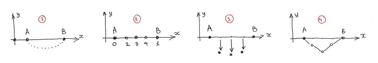
The task: having two source points A and B build a hanging curve between them.

The high-level solution overview:

We would assume that source points are located on the X-axis, at some distance from the origin. We would use Y-axis to move new points down and we would skip the Z-axis for simplicity.

If we think a bit of how the final goal could be achieved step by step, we can note some obvious statements first. We can retrieve the source points position values. We would need to create a certain amount of new points to represent the arc curve and build polygon on top of them. We would need to move those points to a proper position in XY space.

Let's organize our thoughts into the algorithm:

• First, we will create a certain number of points between points A and B.
  We would need to place new points on the equal distance one from another and from the source points. Since our initial anchor points have numbers 0 and 1, our new points will get 2, 3, 4, etc. indexes.
• Next, we will move each new point down on its own value to shape the arc curve.
  The value should rise from the first new point until we reach the middle point, then the value should decrease in the same way until we reach the last new point.
• And finally, we will connect points with polygons to create geometry.

Prepare the scene: create a line SOP in geometry context, orient it along with X-axis, set the number of points to 0, create Attribute Wrangle node after, set the "Run Over" parameter to Detail. We will have our points A and B with indexes 0 and 1 correspondingly.

Creating inbetween points

First, let's store our source anchor point position values in variables and define the number of points we will create between A and B with a UI slider:

vector A = point(0, "P", 0);
vector B = point(0, "P", 1);
int number_of_points = chi('number_of_points');

The point(<input>, <attribute_name>, <point_number>) VEX function returns the value of a point position attribute "P" for point number 0 or 1 for the geometry connected to the first (0) input of a Wrangle node.

Point position is a vector data type {position X, position Y, position Z} so we keep it in a vector variables A and B.

Let's start from the simplest case and create only one new point: set "Number Of Points" attribute to 1.

How we can create the required number of points? When we need to repeat an action (or set of actions, like create a point and define its position) a certain number of times (which is the number of points we want to create), we need to use loop statement:

for(start from; stop at; increment){
   action A;
   action B;
}

For a better understanding of loops, let our first action would be a print statement, which will output the number of iteration to the Houdini Console:

vector A = point(0, "P", 0);
vector B = point(0, "P", 1);
int number_of_points = chi('number_of_points');

for(int iteration=0; iteration<number_of_points; iteration++){
    printf('iteration number = %s\n', iteration);
}

This code will iterate from 0 to 1 (the number of points we set in UI) and output the iteration index to console. The iteration++ is a "syntaxis sugar" for iteration = iteration + 1 statement and means the step of iterations is equal to 1.

Inside the loop body, between { ... } where we currently have the print statement, we will place the code for the new point creation, which will be repeated as many times as many new points we set in the "Number Of Points" parameter.

Change the "Number Of Points" in a Wrangle UI and examine printed results in Houdini Console to see how this basic construction works. Clear console before each value change to isolate each loop execution.

Creating a point with VEX is simple, we need to provide 0 as a first argument and point position (vector value) as a second argument to the addpoint() VEX function.

To create new points we can define their position as a vector variable set to {0, 0, 0}:

vector A = point(0, "P", 0);
vector B = point(0, "P", 1);
int number_of_points = chi('number_of_points');

for(int iteration=0; iteration<number_of_points; iteration++){
   vector point_position = {0, 0, 0};
   addpoint(0,point_position);
}

Now we have a new point created at the origin. If we raise the "Number Of Points" value more points will be added to the same location. How we can evenly distribute all new points between original points A and B? Let's think about adding one point C for now.

After point C were created, we would have 4 points to operate:

• origin point 0
• source point A
• created point C
• source point B

Points define segments:

• segment 0A,
• segment AB,
• segment AC
• segment CB

Let's mark all segments between the new points as S.

We know the A and B point positions (we can get them with point() vex function by point indexes). We need to calculate the point C position to create it in a proper location using known values.

If we want point C to be located at the same distance from A and B, we should divide segment AB into two equal parts:
S = segment AB / 2.

See what will happen when we will raise the number of new points:

Having 2 new points: S = segment AB / 3.
Having 3 new points: S = segment AB / 4.
Having 4 new points: S = segment AB / 5.

This is an obvious pattern which can be expressed as: the length of segment S is equal segment AB/(number of points + 1)

We know, that segment AB = segment 0B - segment 0A, so: segment S = (segment 0B - segment 0A)/(number of points + 1)

Which is the same as: segment S = (position B - position A)/(number of points + 1),

Awesome, now we know how to calculate the length of segments between each new point. Next, let's take a look at how we can get coordinates of new points (C, D, E, etc.) through the segment length:

Point C located away from the origin on a distance of segment 0A + segment AC, and hence position C = position A + segment S.

Having 2 new points: position C = position A + S, position D = position A + S + S
Having 3 new points: position C = position A + S, position D = position A + S + S, position E = position A + S + S + S

We can identify another pattern here: new point position = position A + segment S * (iteration number + 1)

Now, when we have a formula to calculate the new points coordinates, it is easy to implement it in VEX:

vector A = point(0, "P", 0);
vector B = point(0, "P", 1);
int number_of_points = chi('number_of_points');

for(int iteration=0; iteration<number_of_points; iteration++){
    vector segment = (B - A)/(number_of_points + 1);
    vector point_position = A + segment*(iteration + 1); 
    addpoint(0,point_position);
}

Here, with the help of basic math, we have calculated position values for each newly created point using known data: source point positions, amount of new points, and iteration number inside the loop function.

Moving points down along Y-axis.

Let's solve the next sub-task and move new points down individually.

Without going deep into vectors (and our points are vectors) we should realize that in order to move point we need to add or substaract a number from this vector.

We need to develop another formula to create a required arc shape. And developing formula means that we will calculate unknown values from established data. Same as we just did with positioning new points, we calculate a new position based on iteration number of a loop, quantity of points, and source point positions. The art of building necessary dependencies.

As we learn from the sine example, we can use point X position as input to a sine function to shift Y positions to create an arc:

vector A = point(0, "P", 0);
vector B = point(0, "P", 1);
int number_of_points = chi('number_of_points');

for(int iteration=0; iteration<number_of_points; iteration++){
    vector segment = (B - A)/(number_of_points + 1);
    vector point_position = A + segment*(iteration + 1); 
    
    point_position.y -= sin(point_position.x*3.1416);
    
    addpoint(0, point_position);
    
}

The issue with this solution is that if we would move the source points A and B in 3D space away from the origin the arc will brake because the sine function remains in place. Same as when you using procedural texture for the object shading, if you move your objects, textures will slide on the surface, so we need to tie somehow texture to the geometry.

Another option would be to use the iteration numbers instead of the X point position and develop a custom formula instead of a sine function usage.

Let's create a direct dependency between the Y position and iteration number. First, subtract an arbitrary constant number 0.1 from the Y coordinate of new points:

vector A = point(0, "P", 0);
vector B = point(0, "P", 1);
int number_of_points = chi('number_of_points');

for(int iteration=0; iteration<number_of_points; iteration++){
    vector segment = (B - A)/(number_of_points + 1);
    vector point_position = A + segment*(iteration + 1); 
    
    point_position.y -= 0.1;
    
    addpoint(0, point_position);
    
}

Nice, all new points jump down on 0.1 units. Now let them jump on individual value related to iteration number:

point_position.y -= 0.1 * iteration;

The first new point does not moves because the first iteration is 0, let's pick up the first point:

point_position.y -= 0.1 * (iteration + 1);

Ok, this not the final result we are looking for, but it's a good foundation. Our points are going down because the shift value increases each iteration. Next, we need to change the behavior so, that the shift value will start to decrease after we reach the central point.

Since we are using iterations to build points we can say that we need to find the center of iterations, so we just need to divide the number of iterations on 2. If we have an even number of new points, the center would not be a whole number, so we will use float data type to store result:

float iteration_center = number_of_points/2.0;

To check if it's working, let's shift our points only if they are created before the middle iteration:

vector A = point(0, "P", 0);
vector B = point(0, "P", 1);
int number_of_points = chi('number_of_points');
float iteration_center = (number_of_points)/2.0;

for(int iteration=0; iteration<number_of_points; iteration++){
    vector segment = (B - A)/(number_of_points + 1);
    vector point_position = A + segment*(iteration + 1); 
    
    if(iteration < iteration_center)
        point_position.y -= 0.1 * (iteration + 1);

    
    addpoint(0, point_position);
}

To decrease the shift on Y axis, we will add the value instead of substraction:

vector A = point(0, "P", 0);
vector B = point(0, "P", 1);
int number_of_points = chi('number_of_points');
float iteration_center = (number_of_points)/2.0;

for(int iteration=0; iteration<number_of_points; iteration++){
    vector segment = (B - A)/(number_of_points + 1);
    vector point_position = A + segment*(iteration + 1); 
    
    if(iteration < iteration_center )
        point_position.y -= 0.1 * (iteration + 1);
    else
        point_position.y += 0.1 * (iteration + 1);

    
    addpoint(0, point_position);
}

Points started to go up after reaching the center point but it looks like the shift values are higher than we need.

This is happening because after reaching the center point we starting a new set of calculations to reverse the shift direction, but the iteration number continues from the previous steps. So we need to compensate this jump and shift iteration flow after the center. The value of shift would be the number of points we create:

point_position.y += 0.1 * (iteration - number_of_points);

Let's also replace hardcoded increment value with a new float variable "distance":

vector A = point(0, "P", 0);
vector B = point(0, "P", 1);
int number_of_points = chi('number_of_points');
float iteration_center = (number_of_points)/2.0;
float distance = chf('distance');

for(int iteration=0; iteration<number_of_points; iteration++){
    vector segment = (B - A)/(number_of_points + 1);
    vector point_position = A + segment*(iteration + 1); 
    
    if(iteration < iteration_center )
        point_position.y -= distance * (iteration + 1);
    else
        point_position.y += distance * (iteration - number_of_points);
    
    addpoint(0, point_position);
}

We are almost there:

The only thing we need to adjust is a linear behavior of the setup. Currently, each new point is shifted on the same value as the rest of all new points. To get a smoothed curve we need another formula to modify the shift value individually for each point. This value should be dependent on the distance from the center of new points (the closest point to the center should have less shift, e.g. adjusted on a higher value), hence the iteration number could be used here as well.

In other words, we need to scale our points (which are vectors) down closer to center, and to scale vector we need to multiply or divide it by a certain number.

To adjust the shift value we will multiply the Y position by an arbitrary float number (let's name it "curvature"), dependent on an iteration number. Let's just try the same formula:

int number_of_points = chi('number_of_points');
float iteration_center = (number_of_points)/2.0;
float distance = chf('distance');
float curvature = chf('curvature');

for(int iteration=0; iteration<number_of_points; iteration++){
    vector segment = (B - A)/(number_of_points + 1);
    vector point_position = A + segment*(iteration + 1); 
    
        if(iteration < iteration_center ){
            point_position.y -= distance * (iteration + 1);
            point_position.y *= curvature * (iteration + 1);
        }else{
            point_position.y += distance * (iteration - number_of_points);
            point_position.y *= curvature * (iteration - number_of_points);
            }
    
    addpoint(0, point_position); 
}

The direction is correct, the correlation between point distance to the center and Y position is not linear any more, although we need some modifications:

int number_of_points = chi('number_of_points');
float iteration_center = (number_of_points)/2.0;
float distance = chf('distance');
float curvature = chf('curvature');

for(int iteration=0; iteration<number_of_points; iteration++){
    vector segment = (B - A)/(number_of_points + 1);
    vector point_position = A + segment*(iteration + 1); 
    
        if(iteration < iteration_center ){
            point_position.y -= distance * (iteration + 1);
            point_position.y *= curvature * (number_of_points - iteration);
        }else{
            point_position.y += distance * (iteration - number_of_points);
            point_position.y *= curvature * (iteration + 1);
            }
    
    addpoint(0, point_position); 
}

That's an arc we wanted to get, awesome! Finally, let's connect our point with polygon lines. The addprim() function will do the job.

Connect points with polygons

One of the possible usage of addprim() is addprim(<geohandle>, <polygon_type>, <point_number_1>, <point_number_2>) which will build a polygon between to points. We would need a polyline polygon type since the resulting shape is open. We would build all lines in three steps, for the first pair of points, for the last pair of points, and for the rest of the remaining points.

First is the most obvious and easy, we need a line between point A (number 0) and first new point (number 1):
addprim(0, 'polyline', 0, 2);

The last pair of points would be created between the last of new points and the point B (which has an index of 1):
addprim(0, 'polyline', number_of_points + 1, 1);

All new points could be connected:
addprim(0, 'polyline', iteration+1, iteration+2);

Also, to avoid redundant polygons creation we need to run addprim() function for each of three steps only in the part of the loop it needs to be executed. E.g. the first and the last lines should be created only once, and the first and the last iterations is a proper place for execution:

if(iteration==0) 
    addprim(0, 'polyline', 0, 2); 
if(iteration==number_of_points-1)
    addprim(0, 'polyline', number_of_points+1, 1);  

The new points could be created between the first and the last iterations:

if(iteration!=0 && iteration!=number_of_points)
    addprim(0, 'polyline', iteration+1, iteration+2); 

And the final solution:

vector A = point(0, "P", 0);
vector B = point(0, "P", 1);

int number_of_points = chi('number_of_points');
float iteration_center = (number_of_points)/2.0;
float distance = chf('distance');
float curvature = chf('curvature');
    
for(int iteration=0; iteration<number_of_points; iteration++){
    vector segment = (B - A)/(number_of_points + 1);
    vector point_position = A + segment*(iteration + 1); 
    
    if(iteration < iteration_center ){
        point_position.y -= distance * (iteration + 1);
        point_position.y *= curvature * (number_of_points - iteration);
    }else{
        point_position.y += distance * (iteration - number_of_points);
        point_position.y *= curvature * (iteration + 1);
        }
    
    addpoint(0, point_position);
    
    if(iteration==0) 
        addprim(0, 'polyline', 0, 2); 
    if(iteration!=0 && iteration!=number_of_points)
        addprim(0, 'polyline', iteration+1, iteration+2); 
    if(iteration==number_of_points-1)
            addprim(0, 'polyline', number_of_points+1, 1);  
}

Ramp control alternative

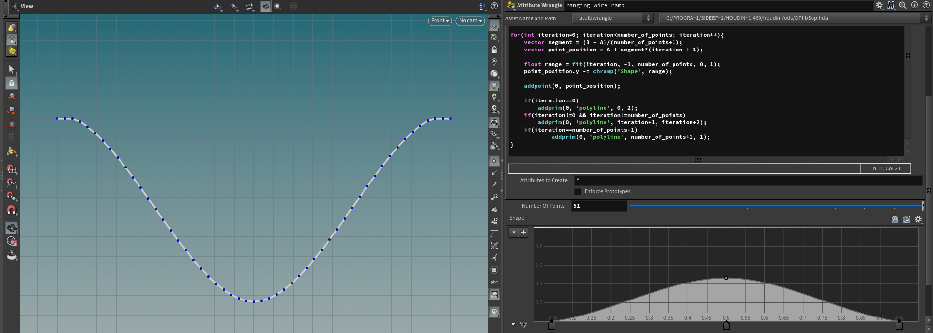
Another option for defining the shape of the curve is using ramp control. In our setup above we rely on the for-loop execution by making dependency between the iteration step and other parameters. So we shift point on Y-axis depending on the iteration number. The higher iteration number leads to higher shift value. Then we modify the iteration flow to get the desired result, we found the center of iterations and change behavior after we reach this point.

We can modify iteration flow in another way — with chramp() function feeding iteration number as input to the ramp. The ramp is working in the range of 0 to 1, so we need to fit our iteration range to required before using it as a ramp input:

vector A = point(0, "P", 0);
vector B = point(0, "P", 1);

int number_of_points = chi('number_of_points');
float iteration_center = (number_of_points)/2.0;
float distance = chf('distance');
float curvature = chf('curvature');
    
for(int iteration=0; iteration<number_of_points; iteration++){
    vector segment = (B - A)/(number_of_points + 1);
    vector point_position = A + segment*(iteration + 1); 
    
    float range = fit(iteration, -1, number_of_points, 0, 1);
    point_position.y -= chramp('Shape', range); 
    
    addpoint(0, point_position);
    
    if(iteration==0) 
        addprim(0, 'polyline', 0, 2); 
    if(iteration!=0 && iteration!=number_of_points)
        addprim(0, 'polyline', iteration+1, iteration+2); 
    if(iteration==number_of_points-1)
            addprim(0, 'polyline', number_of_points+1, 1);  
}

With this setup you will be able to control the shape of the wire with a ramp curve which is more pleasant then sliders but tricky to use if you will need tons of wires with different settings.

Checker

This section inspired by Main Road lookdev classes

Here we will procedurally build a checker using a combination of floor function and a modulus operator (which is an equivalent of the fraction function). You may need to read about functions to be able to follow this tutorial.

At a very high level, the solution would be: build equal-sized black and white stripes (values of 0 and 1), then we will periodically shift a part of each stripe, pally to geometry color.

The diagonal line @P.y = @P.x is a good foundation. Let's make a periodic pattern from it with a modulus:

// Saw pattern with modulus
@P.y = @P.x % 1;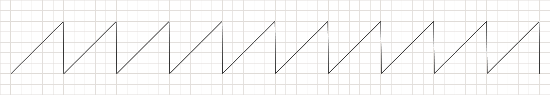

Now, our diagonal line is repeated several times and looks like a saw, a simple repetitive pattern! Let's modify the base pattern further. Scale it twice and pass through the floor function:

// Floor a saw pattern
@P.y = floor(@P.x % 2);

Floor converts float numbers to integers. Applied to any shape it will flatten all diagonal lines to the value of the smallest integer.
Any point position in the range [0-0.99(9)] becomes 0, in range [1-1.99(9)] becomes 1, etc.
Because our initial saw was in range 0-1 (the lowest and highest value of @P.y) we have to scale it up twice to get one repetitive step. Try @P.x % 3 you will get 2 steps and so on.

This shape applied as color gives us stripes! Lets take a look at it, plug a Grid SOP into Attribute Wrangle instead of a line. Set Grid rowsandcolumns` to 1000. Modify color instead of a Y position and see our 0 and 1 values:

// Stripe
@Cd = floor(@P.x % 2);

It was easy, right? Now the fan part. We can create stripes along Z coordinate and add them together getting pattern with 0, 1 and 2 values:

// H and V tripes
@Cd = floor(@P.x % 2) + floor(@P.z % 2);

And clump the result with modulus:

// Checker
@Cd = (floor(@P.x % 2) + floor(@P.z % 2)) % 2;

Before % 2we have a repetition of 0, 1, 2 values: 0,1,2,0,1,2,0,1,2, ...
After modulus 0 and 1 remains as is and 2 becomes 0, so we get 0,1,0,1,0,1,0,1, ...

Another, more tricky solution is to periodically shift a portion of the stripes.
Return to @Cd = floor(@P.x % 2); expression which is equals to @Cd = floor(@P.x) % 2;

Try to add a small number to an argument:
@Cd = floor(@P.x + 0.1) % 2;, @Cd = floor(@P.x + 0.2) % 2;, @Cd = floor(@P.x + 0.3) % 2;
Notice how stripes are sliding left. What will happen if we add a parametric value instead of a constant?

Lets add the Z position. Each point of a stripe will slide on its own value, wchich is defined by @P.z coordinate:

// Taper stripes
@Cd = floor((@P.x + @P.z) % 2);

Obviously, now we need to make those diagonal lines stepped as well, as we did the first time. So we have to floor the Z position input:

// Checker
@Cd= floor((@P.x + floor(@P.z))) % 2;

And a couple of other checker options:

// Checker with fraction
@Cd= floor((frac(@P.x+floor(@P.z*2)*0.5))*2);

// Checker with a sine
@Cd = floor(sin(@P.z + floor(sin(@P.x)) *3.1416 ) + 1); 

Polar checker

In the Sine section we met with polar coordinates, another way to define the position of a point in space.

We can modify our input value more to achieve more complex patterns. Let's take our stripes @Cd = floor(@P.x % 2); and convert point position coordinates from default cartesian to polar before feeding them to the floor function:

// Convert cartesian coords for P to polar
float radius = sqrt(@P.x*@P.x + @P.y*@P.y + @P.z*@P.z);
float u = atan2(@P.y, @P.x) + M_PI;
float v = acos(@P.z/radius)/M_PI;
vector polar_position = set(v,u,radius);

// Polar stripes Z
@Cd = floor(polar_position.z % 2);

The code to convert cartesian coordinates to polar was found in the documentation for the "to_Polar" VOP node.

// Convert cartesian coords for P to polar
float radius = sqrt(@P.x*@P.x + @P.y*@P.y + @P.z*@P.z);
float u = atan2(@P.y, @P.x) + M_PI;
float v = acos(@P.z/radius)/M_PI;
vector polar_position = set(v,u,radius);

// Polar stripes X
float num = 12;
@Cd = floor(num*polar_position.x % 2);

And combining those two we can get radial checker:

@Cd = (floor(polar_position.z % 2) + floor(polar_position.x*12 % 2)) % 2;

Blur

If you don`t like the pattern you get above, you can blur it a bit. Drop another wrangle after your checker:

// Get point numbers (closest to current point) in a certain radius to array
int colsest_points[] = pcfind(0, 'P', @P, chf('radius'), 100);

// Add color valuers for the closest points togather
vector added_color;
foreach(int point; colsest_points){
    added_color+= point(0, "Cd", point);
    }

// Divide by number of points to get avarage color
vector avarage_color = added_color/len(colsest_points);

@Cd = avarage_color;

Vectors

Ok, at this point for the better understanding we might need to look back on the history of math.

We are familiar with math from a very early age and we use to know it as a complete and complex field. We miss the point of how it was born and developed and hence we rarely deeply understanding the miscellaneous math concepts aside from basic arithmetic operation like addition or multiplication.

Let's try to learn math, vectors in particular, from the opposite side we use to: recall the tasks that humanity needed to solve, how those tasks evolved and how this evolution force to develop more advanced mathematical tools.

Numbers

People use to collect different items back in time when we barely can call them humans, it was necessary for survival.

Several apples were just an overall bunch until the moment we start counting the content of a bunch. So we start to recognize the distinction between the different amounts of items: one from two, two from three, three from fore, etc. Then we name those amounts like one, two, three, etc. Next, we gave a name to each number.

Later each number got its own symbol. But at some point, this system becomes hardly manageable:

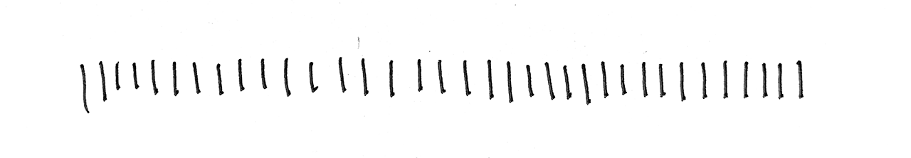
The new way of representing an infinite amount of items with a limited amount of symbols was invented: the positional notation. Say, we have ten symbols to represent our numbers 0, 1, 2, 3, 4, 5, 6, 7, 8, 9. Why ten? Probably because we have ten fingers. It is called a decimal system, but we could use any other amount of symbols. For example, using only two symbols we would have a binary system and it is also a very powerful tool for computation, probably you know that all computer logic built on top of the binary system.

The core idea of positional notation is that to represent any number you have a bucket of certain capacity (10 for decimal and 2 for the binary system). If the number, that you are trying to represent is bigger then a bucket side, the bucket will be completely filled, bucket capacity (e.g. 10 or 2) would be subtracted from the original number, the new bucket with extended capacity (it would be 10 or 2 times bigger for decimal or binary) on the left side from the first bucket would be created, and everything that is left from the original number after subtraction would be placed to this new bucket. If the leftovers are still exceeding the capacity of a new bucket we will create one more bucket which is again 10 (or 2) times bigger then a previous and so on. We are using this system now and I hope everyone is more or less understanding how it is working.

In order to implement a positional notation, humans have to invent a zero first. It might look like an obvious solution today but indeed, back in time, it was not a trivial invention and a huge step forward.

TBD...

VEX next steps

Check VEX snippets for more VEX examples.