COMP7707 / COMP7077 – Assignment 3

Real-time IoT Weather Anomaly Analytics Prototype

System Design & Implementation
Dataset: SGSC_Weather_Sensor_Data.csv (Southern Grampians Weather Sensors)

---

1. Project Overview

This repository implements a real-time IoT analytics prototype for weather anomaly detection.

Main components:

• prototype.py

  • Loads and cleans a public IoT weather dataset
  • Trains Isolation Forest (IF) and a Deep Autoencoder (AE)
  • Simulates real-time streaming and writes results to stream_output.csv

• app.py

  • A Streamlit dashboard that continuously reads stream_output.csv
  • Visualises live sensor trends
  • Highlights anomaly points from both models
  • Shows basic KPIs and an anomaly table

The goal is to show a clear offline → online pipeline:
historical training + model building, then real-time anomaly scoring and monitoring.

---

2. Dataset

• Source: Southern Grampians Shire Council (SGSC) Weather Sensor Data – data.gov.au
• Local file: SGSC_Weather_Sensor_Data.csv (auto-downloaded if missing)
• Download URL: defined as DATA_URL in prototype.py

Time information in the raw dataset is stored in a numeric field with the format YYYYMMDDHHMMSS,
sometimes as integers, sometimes as scientific notation (e.g. 2.01806E+13).

prototype.py:

• Parses this field into a proper datetime column
• Filters the data into a configurable time window (default 2018–2021)

---

3. Repository Structure

• prototype.py – Offline training + real-time streaming (IF + AE)
• app.py – Streamlit dashboard for live anomaly visualisation
• SGSC_Weather_Sensor_Data.csv – Local cache of raw dataset (auto-downloaded if absent)
• stream_output.csv – Streaming output consumed by the dashboard (generated at runtime)

---

4. System Architecture

4.1 Data Preparation (Offline)

1. Download and cache the SGSC dataset if needed.
2. Standardise column names (lowercase, stripped).
3. Locate and parse the time / timestamp column:
   • Convert YYYYMMDDHHMMSS (including scientific notation) to datetime.
4. Filter records between YEAR_START and YEAR_END (defaults: 2018–2021).
5. Select numeric sensor features, for example:
   airtemp, relativehumidity, windspeed, solar,
   vapourpressure, atmosphericpressure, gustspeed, winddirection.
6. Handle missing values using forward/backward fill.
7. Optionally downsample to SAMPLE_SIZE rows for a faster demo.

4.2 Model Training (Offline)

Using the historical window (early part of the time-ordered data):

• Train–stream split

  • Split in temporal order with TRAIN_RATIO (e.g. 70% train, 30% stream).

• Isolation Forest (IF)

  • Implemented with sklearn.ensemble.IsolationForest.
  • Key hyperparameters:
    • contamination – expected anomaly proportion (e.g. 0.05)
    • n_estimators – number of trees
  • Output flag per record:
    • IF_Flag = 1 if predicted as an outlier (-1), else 0.

• Autoencoder (AE)

  • Fully-connected encoder–decoder network:
    • Input = scaled sensor features (StandardScaler)
    • Latent bottleneck to compress normal patterns
  • Training configuration:
    • Optimiser: Adam
    • Loss: MSE reconstruction loss
    • AE_EPOCHS, AE_BATCH_SIZE, AE_LR control training length and speed.
  • Threshold:
    • Compute reconstruction error on the training set
    • Threshold = mean(error) + 3 × std(error)
    • AE_Flag = 1 if current reconstruction error exceeds threshold.

4.3 Streaming Simulation + Dashboard (Online)

• The streaming partition (future window) is processed row by row.

• For each record:

  1. Score with Isolation Forest → IF_Flag.

  2. Scale features and score with the Autoencoder → AE_Flag.

  3. Attach ground-truth label GT_Label (see Section 5).

  4. Append a new row into stream_output.csv:

     Index, Time, <features…>, IF_Flag, AE_Flag, GT_Label

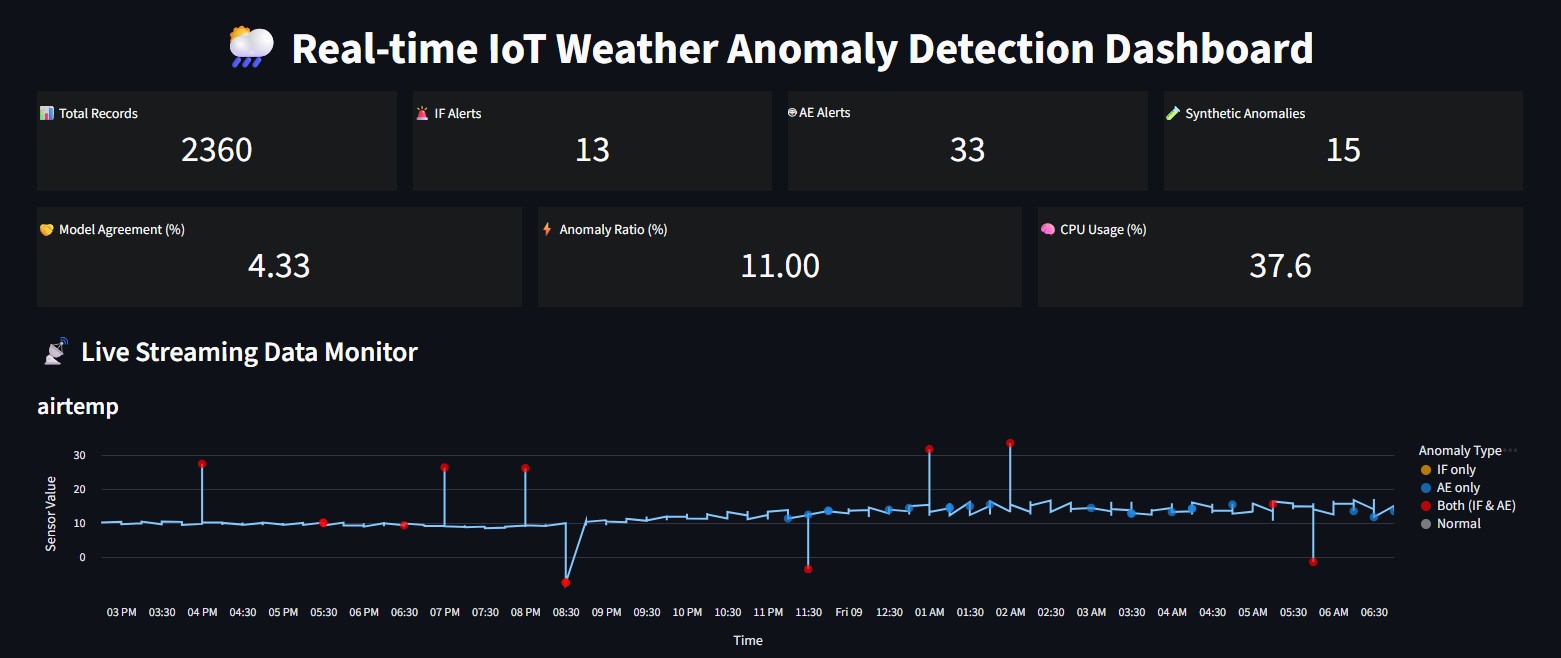
• app.py runs as a Streamlit app and:

  • Continuously reloads stream_output.csv.
  • Shows KPIs (total records, IF/AE alerts, synthetic anomalies, model agreement, anomaly ratio).
  • Plots time-series for selected features with anomaly markers.
  • Displays a table of recent anomaly rows.

---

5. Synthetic Anomalies (GT_Label)

To make anomalies clearer and support simple evaluation:

• prototype.py can inject synthetic anomalies into the streaming set when SYNTHETIC = True.
• A subset of rows (SYNTH_POINTS) is selected at random.
• For each selected row:
  • One or more feature values are perturbed by a multiple of that feature’s standard deviation.
  • A ground-truth label gt_anomaly = 1 is set, and later written as GT_Label in stream_output.csv.

The dashboard uses GT_Label to:

• Count synthetic anomalies,
• Highlight them visually on the plots (e.g. vertical markers),
• Compare IF/AE alerts against a simple ground truth.

---

6. How to Run

6.1 Install Dependencies

Install the required Python packages:

pip install pandas numpy scikit-learn torch streamlit altair psutil

Start the Streaming Engine

python prototype.py

Launch the Streamlit Dashboard

streamlit run app.py

Then open the URL printed in the terminal (normally): http://localhost:8501