PointProcessInference.jl

Fast and scalable non-parametric Bayesian inference for Poisson point processes

Introduction

Poisson point processes are among the basic modelling tools in many areas. Their probabilistic properties are determined by their intensity function, the density λ. This Julia package implements our non-parametric Bayesian approach to estimation of the intensity function λ for univariate Poisson point processes. For full details see our preprint

• S. Gugushvili, M. Schauer, F. van der Meulen, and P. Spreij. Fast and scalable non-parametric Bayesian inference for Poisson point processes. arXiv:1804.03616 [stat.ME], 2018.

Intuitively, a univariate Poisson point processes X, also called a non-homogeneous Poisson process, can be thought of as random scattering of points in the time interval [0,T], where the way the scattering occurs is determined by the intensity function λ. An example is the ordinary Poisson process, for which the intensity λ is constant.

Methodology

We infer the intensity function λ in a non-parametric fashion. The function λ is a priori modelled as piecewise constant. This is even more natural, if the data have been already binned, as is often the case in, e.g., astronomy. Thus, fix a positive integer N and a grid b of points b[1] == 0, b[N] == T on the interval [0,T], for instance a uniform grid. The intensity λ is then modelled as λ(x) = ψ[k] for b[k] <= x < b[k+1].

Now we postulate that a priori the coefficients ψ form a Gamma Markov chain (GMC). As explained in our preprint, this prior induces smoothing across the coefficients ψ, and leads to conjugate posterior computations via the Gibbs sampler. The data-generating intensity is not assumed to be necessarily piecewise constant. Our methodology provides both a point estimate of the intensity function (posterior mean) and uncertainty quantification via marginal credible bands; see the examples below.

Installation

Change julia into the package manager mode by hitting ]. Then run the command add PointProcessInference.

pkg> add PointProcessInference

Usage

In the following example we load the UK coal mining disasters data and performs its statistical analysis via the Poisson point process.

using PointProcessInference
using Random

Random.seed!(1234) # set RNG

observations, parameters, λinfo = PointProcessInference.loadexample("coal")

res = PointProcessInference.inference(observations; parameters...)

The main procedure has signature

 PointProcessInference.inference(observations; title = "Poisson process", T = 1.0, n = 1, ...)

where observations is the sorted vector of Poisson event times, T is the endpoint of the time interval considered, and if observations is an aggregate of n different independent observations (say aggregated for n days), this can be indicated by the parameter n > 1. A full list of parameters is as follows:

function inference(observations;
    title = "Poisson process", # optional caption for mcmc run
    summaryfile = nothing, # path to summary file or nothing
    T0 = 0.0, # start time
    T = maximum(observations), # end time
    n = 1, # number of aggregated samples in `observations`
    N = min(length(observations)÷4, 50), # number of bins
    samples = 1:1:30000, # run for `i in 1:last(samples)` iterations, save coefficients if `i ∈ samples`
    α1 = 0.1, β1 = 0.1, # parameters for Gamma Markov chain
    Π = Exponential(10), # prior on alpha
    τ = 0.7, # Set scale for random walk update on log(α)
    αind = 0.1, βind = 0.1, # parameters for the independent Gamma prior
    emp_bayes = false, # estimate βind using empirical Bayes
    verbose = true
)

Iterates of ψ are the rows of the matrix

res.ψ

High-quality plots

For high quality plotting, the package has a script process-output-simple.jl that visualizes the results with the help of R and ggplot2. After installing the additional dependencies

pkg> add RCall
pkg> add DataFrames

include the script (it is located in the contrib folder, the location can be retrieved by calling PointProcessInference.plotscript())

include(PointProcessInference.plotscript())
plotposterior(res)

The script starts ggplot2 with RCall, and plotposterior expects as its argument the result res returned from inference. For computing the posterior summary measures, the first half of the MCMC iterates is treated as burnin samples.

Example 1

Here, we generate data from a nonhomogeneous Poissson process as follows:

λ0(x) =  (20 + 8*cos(x))
λ0max = 28
obs = PointProcessInference.samplepoisson(λ0, λ0max, 0, 10)

The nonparametric estimator is obtained by running

res = PointProcessInference.inference(obs)

Finally, a default graph is obtained by

include(PointProcessInference.plotscript())
plotposterior(res)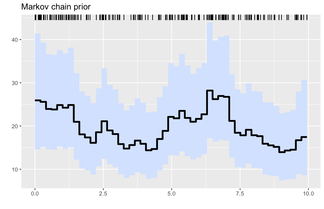

• Illustration: Intensity estimation for the generated data in example 1. The data are displayed via the rug plot in the upper margin of the plot, the posterior mean is given by a solid black line, while a 95% marginal credible band is shaded in light blue.

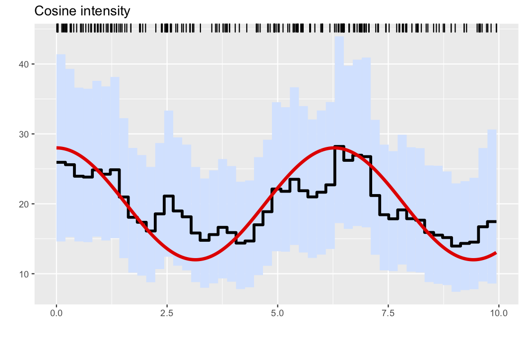
A slightly refined plot, where the true intensity is added to the figure can be obtained by passing the data-generating intensity function as an extra argument.

plotposterior(res;figtitle="Cosine intensity", λ=λ0)

This results in the plot

Example 2

Here, we analyse the well-known coal mining disasters data set.

observations, parameters, λinfo = PointProcessInference.loadexample("coal")
res = PointProcessInference.inference(observations)
plotposterior(res)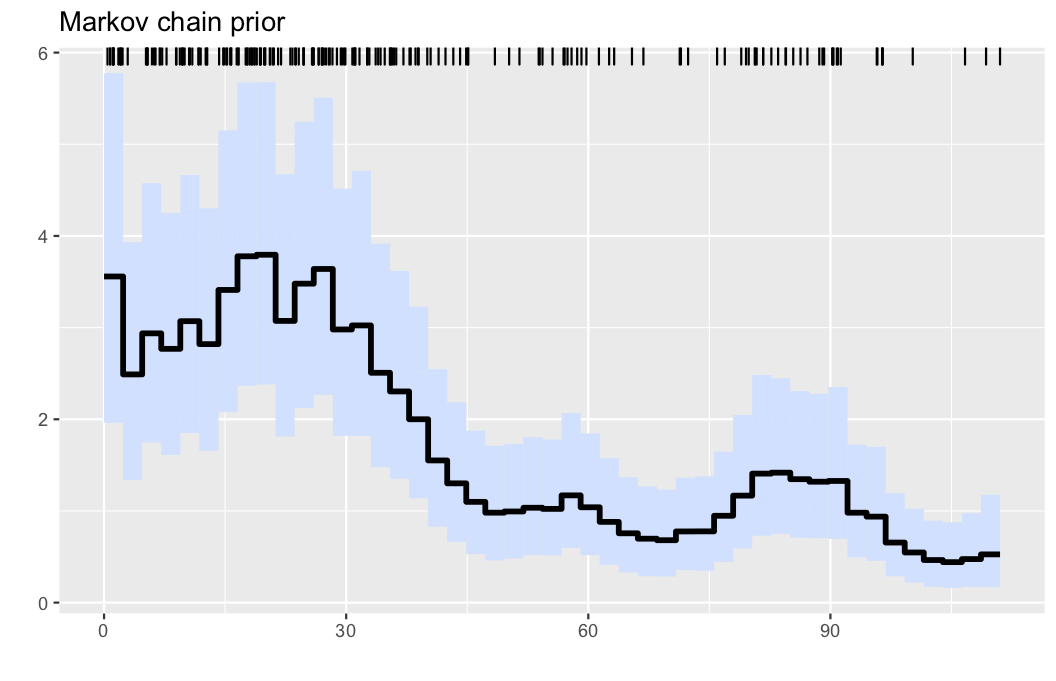

• Illustration: Intensity estimation for the UK coal mining disasters data (1851-1962). The data are displayed via the rug plot in the upper margin of the plot, the posterior mean is given by a solid black line, while a 95% marginal credible band is shaded in light blue.

The horizontal tickmarks can be adjusted, as the offset date of the data, which is March 15, 1851 in this case.

start = 1851+(28+31+15)/365
plotposterior(res; figtitle="Coal mining disasters", offset = start,hortics=1850:10:1960)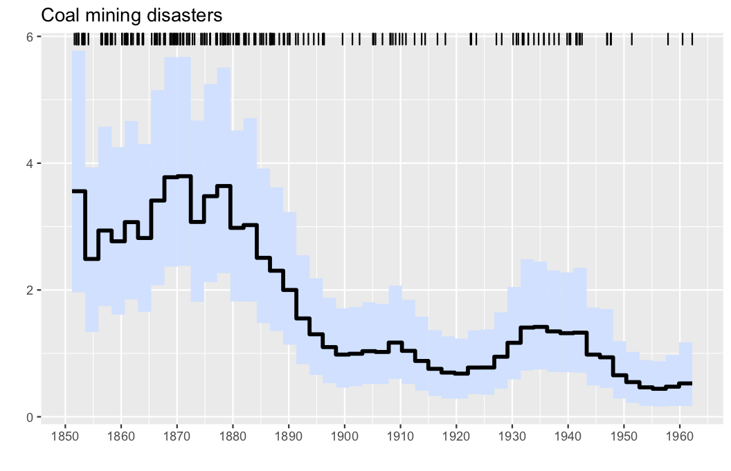

Citing the package

If you use the package in your work, we encourage you to cite it using the following BibTeX code:

@misc{pppjl,
	title = { {PointProcessInference 0.1.0 -- Code and Julia package accompanying the article ``Gugushvili, van der Meulen, Schauer, Spreij (2018): Fast and scalable non-parametric Bayesian inference for Poisson point processes" ({http://arxiv.org/abs/1804.03616})} },
	author = {Gugushvili, Shota and van der Meulen, Frank and Schauer, Moritz and Spreij, Peter},
	year = {2019},
	doi = {10.5281/zenodo.2591395},
	url = {https://doi.org/10.5281/zenodo.2591395},
}