Data simulation
In this workflow, we will generate the BGC domain and class abundance tables, which are needed to create the BGC class abundance models with bgcpred. For this, we will simulate a series of metagenomes based on the Ocean Microbial Reference Gene Catalogue (OM-RGC) (Sunagawa et al., 2015) complete genome sequences. Subsequently, we will compute the number of domain sequences in the simulated metagenomes, and annotate and compute the coverage of the BGC classes in the complete genome sequences (see Figure 1).
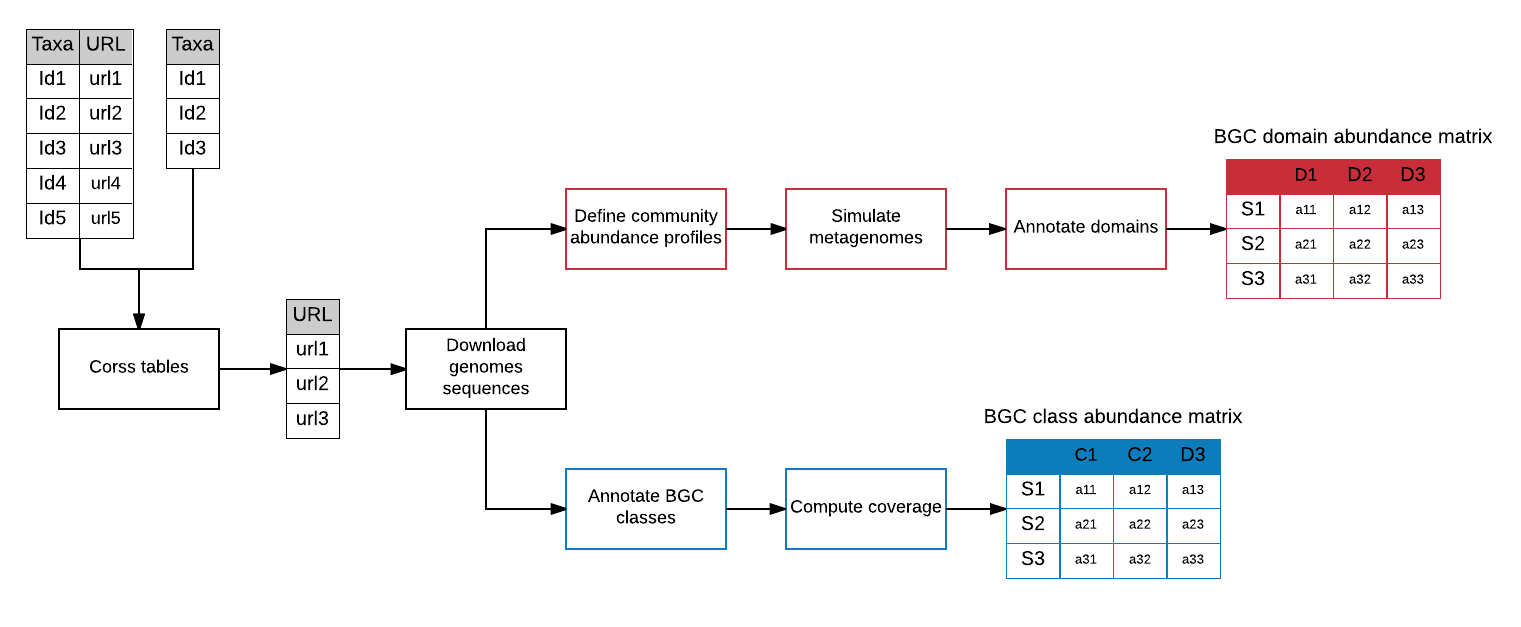 Figure 1. Workflow to create the BGC domain and class abundance matrices based on simulated data.
By using the OM-RGC complete genomes, we aim to construct BGC class abundance models specifically designed for mining marine metagenomic samples. However, you can simulate metagenomes from any type of environment by selecting the appropriate taxonomic profile (e.g. based on OTU tables from previous studies).
We will use the following tools:
SAMtools
BBMap
VSEARCH
EMBOSS
MetaSim
antiSMASH
UProC
FragGeneScan
Bedtools
BiG-MEx
Let's, first of all, create the folders where we will store the data and results.
# make folders
mkdir -p data_simulation/tables
mkdir data_simulation/abundance_tables
mkdir data_simulation/metagenomes
mkdir data_simulation/metagenomes_annot
mkdir data_simulation/ref_genomes
mkdir data_simulation/ref_genomes_annot
mkdir data_simulation/ref_genomes_coverage
And then define the variables with path to the programs we will use. Notice that you will have to substitute "path_to" with your actual path.
# define tools variables
NSLOTS="40"
run_antismash="/path_to/run_antismash"
r_interpreter="/path_to/R"
metasim="/path_to/MetaSim"
reformat="/path_to/bbmap/reformat.sh"
vsearch="/path_to/vsearch"
fraggenescan="/path_to/run_FragGeneScan.pl"
run_bgc_dom_annot="/path_to/bgc_dom_annot.bash"
bwa="/path_to/bwa"
genomecoveragebed="/path_to/genomeCoverageBed"
bamToBed="/path_to/bamToBed"
bedtools="/path_to/bedtools"
samtools="/path_to/samtools"
picard="/path_to/picard.jar"
To create a synthetic metagenome, it is first necessary to construct a database of reference genomes from which to sample. To do this, we will download all complete genomes of the OM-RGC from the GenBank database, following an approach similar to this.
Here we have the OM-RGC taxonomy table and here the assembly_summary.txt table from NCBI. We will download these with wget and store them in the tables folder.
wget --directory-prefix=tables \
https://github.com/pereiramemo/BiG-MEx/wiki/files/OM_reference_genomes_proka.csv
wget --directory-prefix=tables \
ftp://ftp.ncbi.nlm.nih.gov/genomes/refseq/bacteria/assembly_summary.txt
In the following code, we will parse the assembly_summary.txt table to extract the URLs of the OM-RGC complete genomes using awk and egrep. Then, we will use wget once again to download the sequence data.
ASSEM_SUMM="tables/assembly_summary.txt"
ASSEM_SUMM_REDU="tables/assembly_summary_redu.txt"
TAXA_QUERIES="tables/OM_reference_genomes_proka.csv"
TAXA_QUERIES_NAMES="tables/OM_reference_genomes_proka_names.csv"
URLS="tables/OM_reference_genomes_proka_urls.csv"

# format assembly_summary.txt table
awk 'BEGIN {FS="\t"; OFS="\t" } {
  if ( $12=="Complete Genome" && $11=="latest" ) {
    file = $20
    sub(".*/","",file)
    print $8,$20"/"file"_genomic.fna.gz";
  }
}' "${ASSEM_SUMM}" > "${ASSEM_SUMM_REDU}"


# format OM_reference_genomes_proka.csv table
awk 'BEGIN {FS="\t" } {
  if ( NR > 1 ) {
    print $8
  }
}' "${TAXA_QUERIES}" > "${TAXA_QUERIES_NAMES}"

# extract urls
egrep -w -f "${TAXA_QUERIES_NAMES}" "${ASSEM_SUMM_REDU}" | \
cut -f2 > "${URLS}"

# downlaod the data.
wget \
--tries=2 \
--directory-prefix=ref_genomes \
--timeout=120 \
-i "${URLS}"
Before simulating the metagenomes, we have to define a community abundance profile for each metagenome (.mprf files). In this task, we will randomly select between 20 and 80 genomes from the reference database, and assign the genome abundances by sampling from a lognormal distribution with mean 1 and standard deviation of 0.5. It should be noted, that the abundance profiles for MetaSim must specify the abundance of the sequences present in the genomes (i.e. chromosomes and plasmids). For this, we will equally divide a genome abundance into their constituent sequences.
You can change the parameters used here, if you consider other values would be more appropriate in your case.
# we will create a table mapping the genome names to the sequence headers
# and use it in the R script to assign the abundance to each sequence

REF_GENOMES_LIST="tables/ref_genome2headers.list"

# uncompress
gunzip ref_genomes/*.gz

egrep ">" ref_genomes/*.fna | \
sed "s/^ref_genomes\/\(.*.fna\):>\(.*$\)/\1\t\2/" > "${REF_GENOMES_LIST}"


# randomly define abundances
"${r_interpreter}" --vanilla --slave <<RSCRIPT

library("dplyr")

GENOME2HEADER <- read.csv("${REF_GENOMES_LIST}", header = F, sep = "\t", stringsAsFactors = F )
colnames(GENOME2HEADER) <- c("genomes","header")
GENOMES <- unique(GENOME2HEADER[,1])

TABLE <- list()
for ( i in c(1:100) ) {

  set.seed(i)
  RICH <- sample(x = 20:80, size = 1, replace = F)

  set.seed(i)
  GENOME_SUBSAMP_i <- sample(x = 1:length(GENOMES), size = RICH, replace = F)
  GENOME_SUBSAMP <- GENOMES[GENOME_SUBSAMP_i]

  set.seed(i)
  ABUND <- rlnorm(n = RICH , meanlog = 1, sdlog = 0.5 )
  ABUND <- ABUND/sum(ABUND)

  GENOME2ABUND <- data.frame(genomes = GENOME_SUBSAMP, abund = ABUND, stringsAsFactors = F)
  GENOME2HEADER2ABUND <- left_join(GENOME2ABUND, GENOME2HEADER, by = "genomes")

  HEADER2ABUND <- GENOME2HEADER2ABUND %>%
  group_by(genomes) %>%
  mutate( abund2 = (abund/length(genomes)*1000000 ) %>% round() ) %>%
  ungroup() %>%
  cbind(name = "name") %>%
  select(abund2,name,header)

  f <- paste( "abundance_tables/sim_meta_omgrc-", i, ".mprf", sep = "")
  write.table(file = f,x = HEADER2ABUND, quote = T, sep = "\t", row.names = F,
              col.names = F)

}

RSCRIPT

# a formatting detail
sed -i "s/\"name\"/name/"  abundance_tables/*.mprf
Once we have the reference database of complete genomes and the community abundance profiles, we can start the simulations. Each metagenome will be composed of two million mate pair reads of 101bp, with a substitution rate increasing constantly throughout the reads from 1x10⁻⁴ to 9.9x10⁻². With these parameters, we aim to simulate the short read sequences generated by Illumina HiSeq 2000.
We will use MetaSim to simulate the metagenomes. Although, there are other tools that could be used for this (i.e. GemSim, BEAR and NeSSM) we found MetaSim was the most reliable, faster, easy to use and easy to install.
Here you can download the error_model.mcon and here insert_size.txt tables needed for the simulation.
Again, feel free to change the parameters if you consider other values would be more appropriate.
PROFILES=$(ls abundance_tables/*.mprf )
ERROR_MODEL="tables/error_model.mconf"
INSERT_SIZE="tables/insert_size.txt"

# load reference sequences
"${metasim}" cmd --add-files ref_genomes/*.fna

# run simulations
echo "${PROFILES}" | \
while read P; do

  "${metasim}" cmd \
    --empirical \
    --empirical-cfg "${ERROR_MODEL}" \
    --empirical-clones "${INSERT_SIZE}" \
    --reads 2000000 \
    --threads "${NSLOTS}" \
    --empirical-pe-probability 1 \
    --output-dir metagenomes \
    "${P}";

done
Although MetaSim is quite convenient, we will have to add the sequence quality scores "manually".
# compute quality scores from error probabilities
QUAL_SCORE=$( awk 'NR > 2 { Q = -10*(log($1)/log(10));
                   printf("%.0f%s", Q," ")} \
              END { printf "\n" }' "${ERROR_MODEL}" )


echo "${PROFILES}" | \
while read P; do

  PREFIX=metagenomes/$( basename "${P}" .mprf );

  # linearize fasta
  awk 'NR==1 {print ; next} \
  {printf /^>/ ? "\n"$0"\n" : $1} \
  END {printf "\n"}' "${PREFIX}"-Empirical.fna >  "${PREFIX}"_interleaved.fna

  # creat .qual file
  awk -v Q="${QUAL_SCORE}" \
  '$1 ~ />/ { printf "%s\n%s\n", $0,Q } ' \
  "${PREFIX}"_interleaved.fna > "${PREFIX}".qual

  # add quality scores
  "${reformat}" \
  in="${PREFIX}"_interleaved.fna \
  int=t \
  overwrite=t \
  qfin="${PREFIX}".qual \
  out="${PREFIX}".fq

  # clean
  rm "${PREFIX}"_interleaved.fna \
     "${PREFIX}"-Empirical.fna \
     "${PREFIX}".qual
done
Once we have the fastq files, we split them into the R1 and R2 files and merge these two.
echo "${PROFILES}" | \
while read P; do

  PREFIX=metagenomes/$( basename "${P}" .mprf );

  # split into R1 and R2
  cat "${PREFIX}".fq | paste - - - - - - - - | \
  tee >(cut -f 1-4 | tr "\t" "\n" > "${PREFIX}"_R1.fq ) | \
  cut -f 5-8 | sed "s/^\(@r[0-9]\+\)\.2/\1.1/" | tr "\t" "\n" > \
  "${PREFIX}"_R2.fq

  # merge
  "${vsearch}" \
  --threads "${NSLOTS}" \
  --fastq_mergepairs "${PREFIX}"_R1.fq  \
  --reverse "${PREFIX}"_R2.fq  \
  --fastaout "${PREFIX}"_merged.fasta \
  --fastaout_notmerged_fwd "${PREFIX}"_not_merged_R1.fasta \
  --fastaout_notmerged_rev "${PREFIX}"_not_merged_R2.fasta

  # concat
  cat "${PREFIX}"_merged.fasta \
      "${PREFIX}"_not_merged_R1.fasta \
      "${PREFIX}"_not_merged_R2.fasta > "${PREFIX}"_workable.fasta

  # clean
   rm "${PREFIX}".fq \
      "${PREFIX}"_merged.fasta \
      "${PREFIX}"_not_merged_R1.fasta \
      "${PREFIX}"_not_merged_R2.fasta

done
We have the simulations!!! For each metagenome, we have the R1 and R2 fastq files, and the workable fasta file with the merged reads plus the reads that failed get merged (these should represent a very low percentage).
Now we can estimate the domain abundance in each metagenome. In the following code, we will run FragGeneScan to predict the Open Reading Frames (ORFs) and then run_bgc_dom_annt to annotate the domains.
echo "${PROFILES}" | \
while read P; do

  PREFIX=metagenomes/$( basename "${P}" .mprf );
  OUT_PREFIX=metagenomes_annot/$( basename "${P}" .mprf );
  SAMPLE=$( basename "${PREFIX}" )

  "${fraggenescan}" \
  -genome="${PREFIX}"_workable.fasta \
  -out="${PREFIX}" \
  -complete=0 \
  -train=illumina_5 \
  -thread="${NSLOTS}"

  "${run_bgc_dom_annot}" \
  --single_reads "${PREFIX}".faa \
  --intype prot \
  --verbose t \
  --overwrite t \
  --outdir "${OUT_PREFIX}" \
  --sample "${SAMPLE}" \
  --nslots "${NSLOTS}"

done
Just concatenating and reformatting the annotation outputs to have the standard sample x domain abundance matrix.
cat metagenomes_annot/*/counts.tbl > metagenomes_annot/metagenomes_dom_annot.tsv

"${r_interpreter}" --vanilla --slave <<RSCRIPT
library("dplyr")
library("tidyr")

DOM_TABLE <- read.table("metagenomes_annot/metagenomes_dom_annot.tsv", sep = "\t", header = F)
colnames(DOM_TABLE) <- c("sample","domain","count")

DOM_TABLE_WIDE <- DOM_TABLE %>%
                  spread( key = "domain", value = "count", fill = 0)

colnames(DOM_TABLE_WIDE) <- colnames(DOM_TABLE_WIDE) %>%
                            gsub(pattern ="-", replacement = ".")

write.table(x = DOM_TABLE_WIDE, file ="metagenomes_annot/metagenomes_dom_annot_wide.tsv",
            quote = F, row.names = F, sep = "\t")

RSCRIPT
And the BGC domain abundance matrix is finished!!! :) (Remember, these will be our predictive variables later when training the models).
From here on, we will work on the BGC class abundance matrix. Given that we have the complete genome sequences that were used to simulate the metagenomes, we can annotate these with antiSMASH, and then estimate the coverage of each BGC sequence. This should give us something close to the true number and abundance of BGC classes in each metagenome.
# we uncompress the genome data
gunzip ref_genomes/*.gz

# and then run antiSMASH
GENOMES=$(ls ref_genomes/*.fna )

echo "${GENOMES}" | \
while read FNA; do

  "${run_antismash}" \
  "${FNA}" \
  ref_genomes_annot \
  --cpus "${NSLOTS}" \
  --input-type nucl \
  --genefinding prodigal

done
We will create an annotation table where we have the cluster id mapped to the BGC class. We will use this table in the next step.
ls -d ref_genomes_annot/*_asout | \
while read DIR; do

  if [[ -f $(ls "${DIR}"/*.cluster001.gbk) ]]; then

    ls "${DIR}"/*.cluster*.gbk | \
    while read GBK; do
      ACC=$( egrep "LOCUS" "${GBK}" | awk '{print $2}')
      CLUSTER_NUM=$(basename "${GBK}" | sed "s/.*.cluster\([0-9]\+\).gbk/\1/")
      BGC_CLASS=$( egrep "/product=" "${GBK}" | \
                   sed "s/.*\/product=\"\(.*\)\"/\1/")

      GBK_RELAB="${DIR}"/"${ACC}"_"${BGC_CLASS}".cluster"${CLUSTER_NUM}".gbk
      if [[ ! -f "${GBK_RELAB}" ]]; then
        mv "${GBK}" "${GBK_RELAB}"
      fi

      echo -e "${GBK_RELAB}\t${BGC_CLASS}"

    done
  fi
done > ref_genomes_annot/cluster2bgc_class.tsv
Here we will convert gbk to fasta, and edit the header. We will add the BGC class name in the header and file name, so that after estimating the sequence coverage, we can parse each BGC class easily. This is why we needed the annotation table cluster2bgc_class.tsv. Also, we will add a count number, just to keep the ids unique.
cat ref_genomes_annot/cluster2bgc_class.tsv | \
while read LINE; do

  CLUSTER_GBK=$( echo "${LINE}" | cut  -f1 )
  BGC_CLASS=$( echo "${LINE}" | cut -f2 )
  CLUSTER_FASTA=$( echo "${CLUSTER_GBK}" | sed "s/.gbk$//" )"_${BGC_CLASS}.fasta"

  # convert to fasta
  seqret -sequence "${CLUSTER_GBK}" -outseq "${CLUSTER_FASTA}"

  # edit header
  sed -i "s/^>/>cl:${BGC_CLASS}:/" "${CLUSTER_FASTA}"

done
Up to here, we have the annotated BGC class sequences in the complete genomes in fasta format. In this part, we will create a comminity_genomes.tbl table for each metagenome, where we have the names of the complete genome sequences that were selected when defining the community abundance profiles (.mprf files). Remember, this information is not in the .mprf files. These only have the chromosome and plasmid sequence headers specified (not the genome name). We will need this comminity_genomes.tbl table in the next step when we estimate the BGC class sequence coverage.
REF_GENOMES_LIST="tables/ref_genome2headers.list"
PROFILES=$(ls abundance_tables/*.mprf )

# create community genomes table

echo "${PROFILES}" | \
while read LINE; do

  PREFIX=ref_genomes_coverage/$( basename "${LINE}" .mprf );
  mkdir "${PREFIX}"

  awk 'BEGIN { FS="\t" } {
    if ( NR == FNR ) {
      array_header2genome[$2]=$1
      next;
    }
   HEADER=$3
   gsub("\"","",HEADER)
   print array_header2genome[HEADER]
  }' "${REF_GENOMES_LIST}" "${LINE}" | sort | uniq > "${PREFIX}/"community_genomes.tbl

done
Now we will map the simulated metagenome pair read sequences on the BGC sequences. We will use the community_genomes.tbl table to gather all the BGC sequences that should be present in each metagenome.
echo "${PROFILES}" | \
while read P; do

  PREFIX=ref_genomes_coverage/$( basename "${P}" .mprf );
  SAMPLE=$( basename "${P}" .mprf );
  R1=metagenomes/"${SAMPLE}"_R1.fq
  R2=metagenomes/"${SAMPLE}"_R2.fq

  # gather all BGC sequences
  cat "${PREFIX}"/community_genomes.tbl | \
  while read G; do
    cat ref_genomes_annot/"${G/.fna/_asout}"/*cluster*.fasta
  done > "${PREFIX}"/all_bgc_ref.fasta

  # make ids unique
  awk '$1 ~ />/ {sub(">","",$0); n++; print ">"n":"$0; next}; { print $0 }' \
  "${PREFIX}"/all_bgc_ref.fasta > "${PREFIX}"/all_bgc_ref_uids.fasta
  rm  "${PREFIX}"/all_bgc_ref.fasta

  # index
  "${bwa}" index "${PREFIX}"/all_bgc_ref.fasta

   # map
  "${bwa}" mem \
  -M \
  -t "${NSLOTS}" \
  "${PREFIX}"/all_bgc_ref.fasta "${R1}" "${R2}" > \
  "${PREFIX}/${SAMPLE}".sam

  # convert to bam
  "${samtools}" view -@ "${NSLOTS}" -q 10 -F 4 -b \
  "${PREFIX}/${SAMPLE}".sam > "${PREFIX}/${SAMPLE}".bam

  # sort
  "${samtools}" sort  -@ "${NSLOTS}" \
  "${PREFIX}/${SAMPLE}".bam > "${PREFIX}/${SAMPLE}".sorted.bam

  # remove duplicates
  java -jar "${picard}" MarkDuplicates \
        INPUT="${PREFIX}/${SAMPLE}".sorted.bam \
        OUTPUT="${PREFIX}/${SAMPLE}".sorted.markdup.bam \
        METRICS_FILE="${PREFIX}/${SAMPLE}".sorted.markdup.metrics.txt \
        REMOVE_DUPLICATES=TRUE \
        ASSUME_SORTED=TRUE \
        MAX_FILE_HANDLES_FOR_READ_ENDS_MAP=900

  # clean
  rm "${PREFIX}/${SAMPLE}".sam \
     "${PREFIX}/${SAMPLE}".bam \
     "${PREFIX}/${SAMPLE}".sorted.bam

done
Now we can compute the coverage of the BGC classes with the genomecoveragebed tool and the following awk script.
echo "${PROFILES}" | \
while read P; do

  SAMPLE=$( basename "${P}" .mprf );
  PREFIX="${OUTPUT_DIR}"/ref_genomes_coverage/"${SAMPLE}";

  # get coverage histogram
  "${genomecoveragebed}" -ibam "${PREFIX}/${SAMPLE}".sorted.markdup.bam > \
  "${PREFIX}/${SAMPLE}"-coverage.hist

  #############################################################################
  # Compute BGC class coverage as sum( frec*cov )
  # There is no border condition (i.e. END) because the last coverage
  # is always "genome".
  # The coverage of sequences with double classifications
  # (e.g. "terpene-otherks") is repeated for each class.
  #############################################################################


  awk 'BEGIN { FS="\t"; OFS="\t" } {

      if ( $1 != BGC  && NR > 1) {
        BGC_name_only=BGC

        BGC_name_only = gensub(/^[0-9]+:cl:(.*):.*/,"\\\1","",BGC_name_only)

        if (BGC_name_only ~ "-" ) {
          N = split(BGC_name_only,BGC_array,"-")
          for (b in BGC_array) {
            print BGC_array[b],COV
          }
        } else {
          print BGC_name_only,COV
        }
        COV=0
      }

      BGC=$1
      DEPTH=$2
      FRAC=$5
      COV=DEPTH*FRAC + COV

    }'  "${PREFIX}/${SAMPLE}"-coverage.hist > "${PREFIX}/${SAMPLE}"-coverage.table

done
Finally, we concatenate all the *-coverage.tables and do the same formatting as with the domains matrix, so that we have the samples x BGC class abundance matrix.
ls ref_genomes_coverage/sim_meta_*/*-coverage.table | \
while read LINE; do
  SAMPLE=$( basename "${LINE}" -coverage.table );
  sed "s/^/${SAMPLE}\t/" "${LINE}";
done > ref_genomes_coverage/ref_genomes_class_cov.tsv

"${r_interpreter}" --vanilla --slave <<RSCRIPT
library("dplyr")
library("tidyr")

CLASS_TABLE <- read.table("ref_genomes_coverage/ref_genomes_class_cov.tsv", sep = "\t", header = F)

colnames(CLASS_TABLE) <- c("sample","class","coverage")

CLASS_TABLE_WIDE <- CLASS_TABLE %>%
                     group_by(sample, class) %>%
                     summarize( total_coverage = sum(coverage) ) %>%
                     spread( key = "class", value = "total_coverage", fill = 0) %>%
                     ungroup()

colnames(CLASS_TABLE_WIDE) <- colnames(CLASS_TABLE_WIDE) %>%
                              gsub(pattern ="-", replacement = ".")

write.table(x = CLASS_TABLE_WIDE, file ="ref_genomes_coverage/ref_genomes_class_cov_wide.tsv",
            quote = F, row.names = F, sep = "\t")

RSCRIPT
We are finished!!! Now you can import your metagenomes_dom_annot_wide.tsv and ref_genomes_class_cov_wide.tsv tables to R and create your own models with bgcpred as we show it here. Enjoy :)