PICRUSt2 Tutorial (v2.3.0 beta)
Past PICRUSt2 tutorials are listed here.
PICRUSt2 (Phylogenetic Investigation of Communities by Reconstruction of Unobserved States) is a software for predicting functional abundances based only on marker gene sequences.
"Function" usually refers to gene families such as KEGG orthologs and Enzyme Classification numbers, but predictions can be made for any arbitrary trait. Similarly, predictions are typically based on 16S rRNA gene sequencing data, but other marker genes can also be used.
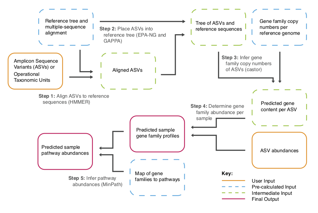
The key steps of the PICRUSt2 pipeline are indicated in the below flowchart.
In this tutorial example 16S rRNA gene sequencing data will be used to generate predictions for EC numbers and MetaCyc pathways.
The most important thing to keep in mind when running PICRUSt2 is that predictions of functional potential are output. This data can be useful for generating hypotheses, but should always be interpreted cautiously especially when focused on a single function or predictions for a single ASV (or OTU). You should read through the key limitations of metagenome inference before proceeding.
The final output tables produced by PICRUSt2 are essentially the read depth per ASV multiplied by the predicted function abundances per ASV. The output is calculated slightly differently depending on the file as described below, but that is the basic idea. Accordingly, the final tables are not output in terms of relative abundance and the abundances per sample will sum to different numbers.
There are many possible ways to analyze the output of PICRUSt2, such as rounding the data and using the ALDEx2 R package. However, no matter what approach you use it is important to keep in mind that the data is compositional. This means that it would be inappropriate to run a Wilcoxon test (for example) on the output table without first transforming the data somehow (e.g. to relative abundance, centred-log ratio transformation, etc.).
You can cite our paper, which is found here.
In addition, PICRUSt2 wraps a number of tools to generate functional predictions from amplicon sequences. If you use PICRUSt2 you also need to cite the below tools.
For hidden state prediction:
PICRUSt2 is only available for Mac OS X and Linux systems (not for Windows unless you are running a Linux emulator). Before running the installation commands below you will need to install Miniconda.
To run this tutorial you will need at least 16 GB of RAM, however you can still run through most of this tutorial with less RAM. The key memory-intensive step is the read placement, which you can avoid by simply downloading the expected output file and proceeding with the tutorial. When running your data you can run the QIIME2 plugin of PICRUSt2 and use SEPP for read placement. Using this approach is much less memory intensive, but currently there are fewer options available for the QIIME2 plugin.
The easiest way to install PICRUSt2 is with bioconda, which will install a new environment which contains all the software needed to run PICRUSt2.
conda create -n picrust2 -c bioconda -c conda-forge picrust2=2.3.0_b
When using conda you need to specifically activate environments to use them:
conda activate picrust2
For this tutorial we will be looking at a dataset that was originally used in a project to determine whether knocking out the protein chemerin affects gut microbial composition. In this mapping file described below the genotypes of interest can be seen: wildtype (WT) and knockout (KO). Also of importance are the two source facilities: "PaloAlto" and "Dalhousie".
Note that this dataset has been greatly simplified for this demonstration. For more details on this dataset check out the publication in PeerJ.
First, download, unzip, and enter the folder of tutorial files:
wget http://kronos.pharmacology.dal.ca/public_files/picrust/picrust2_tutorial_files/chemerin_16S.zip
unzip chemerin_16S.zip
cd chemerin_16S
You should see the three files below when you type ls -1:
metadata.tsv
seqs.fna
table.biom
These files are processed datafiles rather than raw reads. We can take a look at the input FASTA file with less (note that with less you can go back to the terminal by typing q).
less seqs.fna
You should see:
>86681c8e9c64b6683071cf185f9e3419
CGGGCTCAAACGGGGAGTGACTCAGGCAGAGACGCCTGTTTCCCACGGGACACTCCCCGAGGTGCTGCATGGTTGTCGTC
AGCTCGTGCCGTGAGGTGTCGGCTTAAGTGCCATAACGAGCGCAACCCCCGCGTGCAGTTGCTAACAGATAACGCTGAGG
ACTCTGCACGGACTGCCGGCGCAAGCCGCGAGGAAGGCGGGGATGACGTCAAATCAGCACGGCCCTTACGTCCGGGGCGA
CACACGTGTTACAATGGGTGGTACAGCGGGAAGCCAGGCGGCGACGCCGAGCGGAACCCGAAATCCACTCTCAGTTCGGA
TCGGAGTCTGCAACCCGACTCCGTGAAGCTGGATTCGCTAGTAATCGCGCATCAGCCATGGCGCGGTGAATACGTTCCCG
>b7b02ffee9c9862f822c7fa87f055090
AGGTCTTGACATCCAGTGCAAACCTAAGAGATTAGGTGTTCCCTTCGGGGACGCTGAGACAGGTGGTGCATGGCTGTCGT
CAGCTCGTGTCGTGAGATGTTGGGTTAAGTCCCGCAACGAGCGCAACCCTTGTCATTAGTTGCCATCATTAAGTTGGGCA
CTCTAATGAGACTGCCGGTGACAAACCGGAGGAAGGTGGGGATGACGTCAAGTCATCATGCCCCTTATGACCTGGGCTAC
ACACGTGCTACAATGGACGGTACAACGAGAAGCGAACCTGCGAAGGCAAGCGGATCTCTTAAAGCCGTTCTCAGTTCGGA
CTGTAGGCTGCAACTCGCCTACACGAAGCTGGAATCGCTAGTAATCGCGGATCAGCACGCCGCGGTGAATACGTTCCCGG
...
This file contains the Amplicon Sequence Variants (ASVs) of 16S rRNA gene sequences found across the mouse stool samples. The id of each ASV is written on the lines starting with ">", so the id of the first sequence is "86681c8e9c64b6683071cf185f9e3419".
These are the ids produced by the deblur denoising pipeline so the ids of your dataset may look very different depending on what pipeline you ran. For instance, this file could alternatively contain Operational Taxonomic Unit (OTU) sequences; PICRUSt2 is agnostic to which processing pipeline is used for 16S rRNA gene data. However, this file should not contain raw (i.e. non-denoised/unclustered) read sequences. In addition, the header-line for each sequence (lines starting with ">") should only contain the sequence id. If your file has additional information on each header-line following the sequence id see here. Lastly, these sequences should be on the positive strand of the 16S rRNA gene.
The next file is a bit tricky to view since it is a BIOM file which is binary encoded (not easily viewed with a plain-text viewer). We can get a sense of what the first few columns and rows look like by using the following command:
biom head -i table.biom
You should see:
# Constructed from biom file
#OTU ID	100CHE6KO	101CHE6WT	102CHE6WT	103CHE6KO	104CHE6KO
86681c8e9c64b6683071cf185f9e3419	716.0	699.0	408.0	580.0	958.0
b7b02ffee9c9862f822c7fa87f055090	51.0	98.0	96.0	91.0	223.0
663baa27cddeac43b08f428e96650bf5	112.0	29.0	45.0	35.0	75.0
abd40160e03332710641ee74b1b42816	0.0	0.0	0.0	0.0	0.0
bac85f511e578b92b4a16264719bdb2d	56.0	4.0	63.0	131.0	90.0
Notice, that the first column ("#OTU ID") contains the ASV ids in the FASTA file above. The first column of this table needs to match the ids in the FASTA file. The additional columns represent different samples with the counts representing the number of reads within each of those samples. Importantly, the input table should contain read counts rather than relative abundance. You can input a rarefied table, but that is not required.
We can get more information about the rest of the table by using this command:
biom summarize-table -i table.biom
The input tutorial datafiles have already been pre-processed, but there are a few things you should keep in mind for your own data:
-
Depending on the pipeline you used to process your raw 16S data there may be many extremely rare ASVs found across your samples. Such rare ASVs typically only add noise to analyses (especially singletons - ASVs found only by 1 read in 1 sample) and should be removed. Reducing the number of input ASVs will also make PICRUSt2 faster and less memory intensive.
-
Similarly, it is important to check for any low-depth samples that should be removed. These can be identified based on the output of
biom summarize-tableabove. -
The best minimum cut-offs for excluding ASVs and samples varies by dataset since these cut-offs will differ depending on the overall read depth of your dataset.
-
There are many ways to filter a BIOM table, but one easy approach is described in a QIIME2 tutorial.
Now that we have and understand the data we can run PICRUSt2!
The easiest way to run PICRUSt2 is with the picrust2_pipeline.py script,
which you can see here.
This script automatically will run all of the steps that are described below.
However, for the purposes of the tutorial we will run each step individually so
that it is easier to follow.
First make and enter a new folder for writing the PICRUSt2 output files.
mkdir picrust2_out_pipeline
cd picrust2_out_pipeline
When running the below commands you can swap in the number of available cores
for the 1 in -p 1, which will allow many steps to be run in parallel and
speed up the pipeline.
The first step of PICRUSt2 is to insert your study ASVs into a reference tree (details). By default, this reference tree is
based on 20,000 16S sequences from genomes in the Integrated Microbial Genomes
database. The place_seqs.py script performs this step, which specifically:
-
Aligns your study ASVs with a multiple-sequence alignment of reference 16S sequences with HMMER.
-
Find the most likely placements of your study ASVs in the reference tree with EPA-NG.
-
Output a treefile with the most likely placement for each ASV as the new tips with GAPPA.
You can run these steps with this command (1 minute and 13.8 GB of RAM on 1 processor):
place_seqs.py -s ../seqs.fna -o out.tre -p 1 \
              --intermediate intermediate/place_seqs
The required input is the FASTA of the ASV sequences. The key output file is
out.tre, which is a tree in newick format of your study ASVs and
reference 16S sequences. If you do not have enough RAM to run this command locally you can simply download the expected out.tre output file here.
There are extra options (that we could have left out):
-
-p 1indicates how many processors to use. -
--print_cmdsindicates that it should show us the commands that it is running in the background. -
--intermediate intermediate/place_seqsindicates where intermediate files should be saved. Although only the most likely placement is output for each ASV the intermediate files can also be useful for advanced users. You can find these intermediate files inintermediate/place_seqs/, which includes the JPLACE file (intermediate/place_seqs/epa_out/epa_result.jplace) of all potential placements per ASV in the tree.
Note that in this case the output tree should be the same every time you run the command. However, with larger datasets you can run into situations where a single ASV places equally well at many places in the reference tree. This can result in minor variation each time read placement is run meaning it may not be exactly reproducible.
In addition, different ASV placements can sometimes occur when different input ASV sets are specified (i.e. ASV placements can be dependent on the other ASVs being placed). We are currently addressing this issue.
Hidden-state prediction of gene families
There are many approaches for inferring what the likely trait values are for unknown lineages on a phylogenetic tree. PICRUSt2 uses the approaches implemented in the castor R package. The script hsp.py runs this step in PICRUSt2 (see details), which by default will run maximum parsimony. This script predicts the missing genome for each ASV, i.e. it predicts the copy number of gene families for each ASV. Predictions for several gene family databases are possible, but we will restrict predictions to the EC number database to save time. Note that most users will likely also want to predict KEGG orthologs as well. We will also predict the copy number of 16S rRNA gene sequences per ASV for reasons that will become clear at the next step!
The script hsp.py can also output the nearest-sequenced taxon index (NSTI) values for each ASV (specified by the -n option), which correspond to the branch length in the tree from the placed ASV to the nearest reference 16S sequence. This metric is a rough guide for how similar an ASV is to an existing reference sequence. Predictions are more accurate for ASVs that have well-characterized close relatives.
Run hsp.py, which will take 4 min and 1 GB of RAM on 1 processor with this dataset.
hsp.py -i 16S -t out.tre -o marker_predicted_and_nsti.tsv.gz -p 1 -n

hsp.py -i EC -t out.tre -o EC_predicted.tsv.gz -p 1
The output files of these commands are marker_predicted_and_nsti.tsv.gz (download) and EC_predicted.tsv.gz (download). Note that these files are gzip compressed to save space. We can take a look at them using zless -S (zless is like less, but for gzipped files, and the -S option turns off line wrapping so it is easier to see):
zless -S marker_predicted_and_nsti.tsv.gz
You should see this:
sequence        16S_rRNA_Count  metadata_NSTI
20e568023c10eaac834f1c110aacea18        1       0.008994
23fe12a325dfefcdb23447f43b6b896e        1       0.047617
288c8176059111c4c7fdfb0cd5afce64        4       0.44977799999999996
2a45f0b7f68a35504402988bcb8eb7fe        1       0.000101
343635a5abc8d3b1dbd2b305eb0efe32        4       0.5681
...
The first column is the name of ASV, followed by the predicted number of 16S copies per ASVs, followed finally by the NSTI value per ASV. When testing several datasets we found that ASVs with a NSTI score above 2 are usually noise. It can be useful to take a look at the distribution of NSTI values for your ASVs to determine how well-characterized your community is overall and whether there are any outliers.
If you take a look at EC_predicted.tsv.gz you will see a similar table:
sequence        EC:1.1.1.1      EC:1.1.1.10     EC:1.1.1.100    ...
20e568023c10eaac834f1c110aacea18        2       0       3    ...
23fe12a325dfefcdb23447f43b6b896e        0       0       1    ...
288c8176059111c4c7fdfb0cd5afce64        1       0       1    ...
...
In this table the predicted copy number of all Enzyme Classification (EC) numbers is shown for each ASV. The NSTI values per ASV are not in this table since we did not specify the -n option. EC numbers are a type of gene family defined based on the chemical reactions they catalyze. For instance, EC:1.1.1.1 corresponds to alcohol dehydrogenase. In this tutorial we are focusing on EC numbers since they can be used to infer MetaCyc pathway levels (see below).
In the last step we predicted the copy numbers of gene families for each ASV. This output alone can be useful; however, often users are more interested in the predicted gene families weighted by the relative abundance of ASVs in their community. In other words, they are interested in inferring the metagenomes of the communities. This output can be produced by plugging in the BIOM table of ASV abundances per samples that we downloaded at the beginning. There are two steps performed at this stage:
-
The read depth per ASV is divided by the predicted 16S copy numbers. This is performed to help control for variation in 16S copy numbers across organisms, which can result in interpretation issues. For instance, imagine an organism with five identical copies of the 16S gene that is at the same absolute abundance as an organism with one 16S gene. The ASV corresponding to the first organism would erroneously be inferred to be at higher relative abundance simply because this organism had more copies of the 16S gene.
-
The ASV read depths per sample (after normalizing by 16S copy number) are multiplied by the predicted gene family copy numbers per ASV.
The metagenome_pipeline.py script will run these steps (details), which should run in ~5 seconds:
metagenome_pipeline.py -i ../table.biom -m marker_predicted_and_nsti.tsv.gz -f EC_predicted.tsv.gz \
                       -o EC_metagenome_out --strat_out
The --strat_out option indicates that the stratified output file, which is a long-format table that indicates how ASVs contribute ECs, will also be output.
There are several output files created within the EC_metagenome_out directory:
-
EC_metagenome_out/pred_metagenome_unstrat.tsv.gz(download) - overall EC number abundances per sample. -
EC_metagenome_out/pred_metagenome_contrib.tsv.gz(download) - A stratified table in "contributional" format breaking down how the ASVs contribute to gene family abundances in each sample. -
EC_metagenome_out/seqtab_norm.tsv.gz(download) - the ASV abundance table normalized by predicted 16S copy number. -
EC_metagenome_out/weighted_nsti.tsv.gz(download) - the mean NSTI value per sample (when taking into account the relative abundance of the ASVs). This file can be useful for identifying outlier samples in your dataset. In PICRUSt1 weighted NSTI values < 0.06 and > 0.15 were suggested as good and high, respectively. The cut-offs can be useful for getting a ball-park of how your samples compare to other datasets, but a weighted NSTI score > 0.15 does not necessarily mean that the predictions are meaningless.
Take a look at the EC prediction tables with less as before.
zless -S EC_metagenome_out/pred_metagenome_unstrat.tsv.gz
You should see a table like this:
function        100CHE6KO       101CHE6WT       102CHE6WT       ...
EC:1.1.1.1      1432.0  1967.5  1408.5  ...
EC:1.1.1.100    2034.0  2748.16 2443.5  ...
EC:1.1.1.103    0.0     0.0     0.0     ...
This table is similar to the ASV abundance table except that the rows are gene families rather than ASVs. It is important to note that this output is not in relative abundance and even if you input a rarified BIOM table the columns of this table will not sum to the same number!
Now look at the stratified output:
sample  function        taxon   taxon_abun      taxon_rel_abun  genome_function_count   taxon_function_abun     taxon_rel_function_abun
100CHE6KO       EC:1.1.1.1      20e568023c10eaac834f1c110aacea18        26.0    1.9607843137254901      2       52.0    3.9215686274509802
100CHE6KO       EC:1.1.1.1      288c8176059111c4c7fdfb0cd5afce64        25.5    1.9230769230769231      1       25.5    1.9230769230769231
100CHE6KO       EC:1.1.1.1      343635a5abc8d3b1dbd2b305eb0efe32        16.0    1.206636500754148       1       16.0    1.206636500754148
The columns of this file are:
-
sample - The sample ID.
-
function - Function ID (typically gene family or pathway).
-
taxon - Taxon ID (typically an ASV ID).
-
taxon_abun - Abundance of this taxon in the sample. If abundances were normalized by marker gene abundance this will be the normalized abundance, but NOT in terms of relative abundance.
-
taxon_rel_abun - This is the same as the "taxon_abun" column, but in terms of relative abundance (so that the sum of all taxa abundances per sample is 100).
-
genome_function_count - Predicted copy number of this function per taxon.
-
taxon_function_abun - Multiplication of "taxon_abun" column by "genome_function_count" column.
-
taxon_rel_function_abun - Multiplication of "taxon_rel_abun" column by "genome_function_count" column.
One thing to watch out for is that if you want to input this table of ASV contributions to another tool you should not use the --min_reads and --min_samples option to collapse rare ASVs to the RARE category since treating rare taxa as a single taxon would likely be inappropriate for many analyses (this will not happen by default).
This filetype was recently added to PICRUSt2 and is similar to the input required for several programs like BURRITO and MIMOSA. These tools expect the legacy format of this table output by PICRUSt1. To generate this file in legacy format you can run:
convert_table.py EC_metagenome_out/pred_metagenome_contrib.tsv.gz \
                 -c contrib_to_legacy \
                 -o EC_metagenome_out/pred_metagenome_contrib.legacy.tsv.gz
The last major step of the PICRUSt2 pipeline is to infer pathway-level abundances with pathway_pipeline.py (details).
By default this script infers MetaCyc pathway abundances based on EC number abundances, although different gene families and pathways can also be optionally specified. This script performs a number of steps by default, which are meant to be as similar as possible to the approach implemented in HUMAnN2:
- Regroups EC numbers to MetaCyc reactions.
- Infers which MetaCyc pathways are present based on these reactions with MinPath.
- Calculates and returns the abundance of pathways identified as present.
You can run these steps with this command, which should take < 2 min and very little RAM with this dataset:
pathway_pipeline.py -i EC_metagenome_out/pred_metagenome_contrib.tsv.gz \
                    -o pathways_out -p 1
The output of this script are in the pathways_out folder. These include both unstratified (download) and stratified (download) MetaCyc pathway abundances, similar to the EC number tables above. Note that this stratified output was output since a stratified gene family table was input.
This default stratified pathway abundance table represents how much each ASV is contributing to the community-wide pathway abundance and not what the pathway abundance is predicted to be within the predicted genome of that ASV alone. For that output you would need to use the --per_sequence_contrib option, which is more computationally intensive to run since pathways need to be inferred for each individual ASV. As of v2.2.0-b an additional unstratified pathway abundance table will also be output when this option is used based on summing over all contributing sequences in this alternative stratified table (named path_abun_unstrat_per_seq.tsv.gz). A further discussion of the difference between these stratified pathway outputs is found here.
Finally, it can be useful to have a description of each functional id in the output abundance tables. The below commands will add these descriptions as new column in gene family and pathway abundance tables (details):
add_descriptions.py -i EC_metagenome_out/pred_metagenome_unstrat.tsv.gz -m EC \
                    -o EC_metagenome_out/pred_metagenome_unstrat_descrip.tsv.gz

add_descriptions.py -i pathways_out/path_abun_unstrat.tsv.gz -m METACYC \
                    -o pathways_out/path_abun_unstrat_descrip.tsv.gz
Note that the mapping of function ids to descriptions can also be found in the files within this folder of the PICRUSt2 repository: picrust2/picrust2/default_files/description_mapfiles/.
As mentioned above, there are many possible ways to analyze the PICRUSt2 output. STAMP is one tool that can be used that requires no background in scripting languages. This tool is very useful for visualizing microbiome data, but note that there are better alternatives for conducting statistical tests with compositional data (such as the ALDEx2 R package). If you would like to try out STAMP for visualizing the PICRUSt2 output, see here.
No matter what analysis approach you take, you should be aware that results based on differential abundance testing can vary substantially between shotgun metagenomics sequencing data and amplicon-based metagenome predictions based on the same samples. This is especially true for community-wide pathway predictions. Please check out this post and this response to a FAQ for more details.