2. Introduction
Asami is a graph database, which may be a new approach to data management for some users. This page tries to explain what graph data is and how to use Asami to interact with it.
When we refer to a "Graph Database" we are not referring to the sort of graph that we often see in magazines, or are generated from spreadsheets. Instead, the "graph" being referenced here is a branch of mathematics called "Graph Theory". These graphs describe a set of items called "Nodes", which are connected with lines that are called "Edges".
An example of this might be a graph of social connections between people. The people in such a network can be represented by the "nodes" of a graph, and the "edges" can represent the social connections between them.
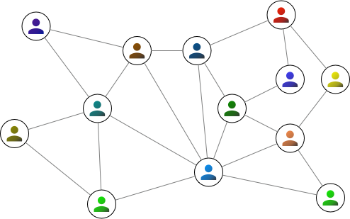
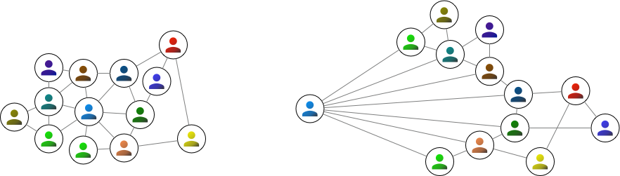
Each node appears once in a graph, regardless of how many connections it may have, and any pair of nodes will only have a single edge between them. Another important thing is that an image of a graph is merely a representation of the data. The location of the nodes and the edges do not matter. Also, edges do not interact in any way, so even if the lines indicating edges cross over each other, this does not mean anything. For instance, the following 2 graphs represent identical data to the above graph:
While many subtleties emerge from this structure, these simple ideas describe the entire foundation of this branch of mathematics!
However, most graph databases (including Asami) add two important features to the above definition: directed edges, and labeling.
A variation on the above graphs is when the edges are given a direction. We can represent this in an image using arrows instead of simple lines. Perhaps this might be used to represent a company hierarchy.
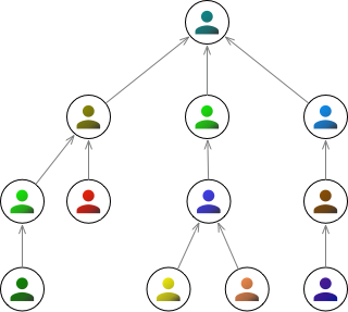
Importantly, having direction on edges means that there can now exist 2 edges between a pair of nodes: one in either direction.
A labeled graph will have labels on both the nodes and the edges. This provides a lot of new possibilities:
- Nodes need not represent the same types of things. They can represent anything: people, organizations, inventory items, account entries – anything at all.
- Multiple edges can connect the same nodes. For instance, a woman who is a mother to someone is also that person's parent. Both of these connections can be represented as distinct labeled edges.
Labeling some of the previous graph, we could get something like this:
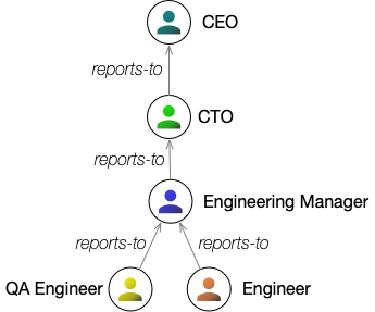
Labeled, directed graphs form the basic structure of graph databases.
Different graph databases make different choices about how they store their graph information. A common approach is for each node in the graph to be an object that has multiple attributes on it. We see this sort of thing in the Neo4J Graph Database.
Using this approach, let's add some details to the organization chart we had a moment ago.

This diagram shows how entities can group a lot of information together in the graph. However, Asami and other graph databases actually break this information down into a basic graph structure. The information is identical, but it just gets managed a little differently.
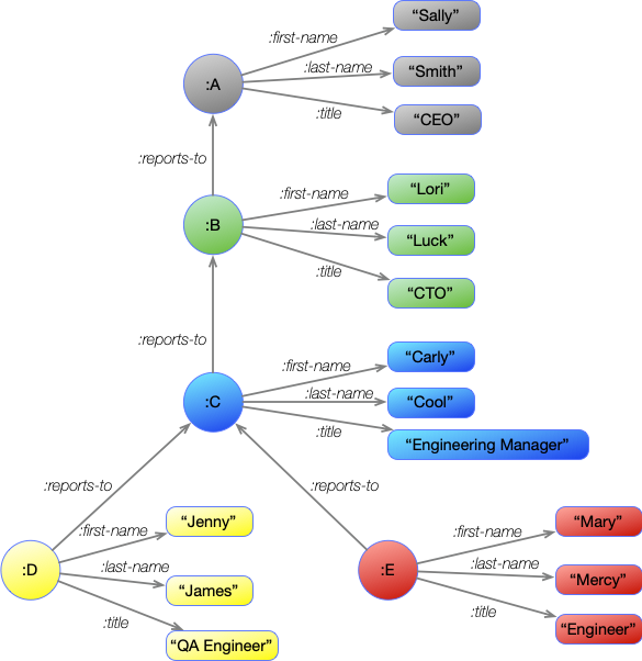
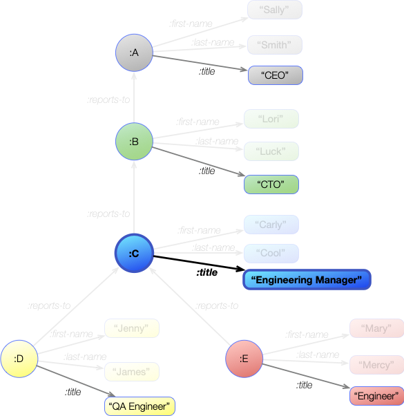
This is identical information as in the previous diagram, but instead of nodes being associated with complex data structures, every node represents only a single unit of information. Some are strings, while others provide a point to represent a group of information. These other nodes also need labels, so they have each been assigned a letter. These labels are often assigned automatically, though the user can choose what they will be.
You may have noticed that the edge and node labels all start with a : character. Asami is a Clojure database, and this is the syntax of a Clojure keyword. Other types of labels can be used, but keywords are very common and easy. We will stick to them here for consistency.
While the graph images above are clear in their structure, they have several limitations. As the amount of information expands, the size of the graph can grow significantly. The details and labels can get lost. For instance, there is no way to provide labels in the following graph without the image becoming enormous.
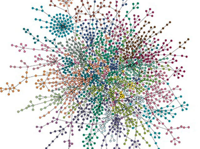
At the same time, the graph information has to be stored in a computer where it can be accessed in an efficient manner. This is done by storing only the information necessary for the graph.
The representation for basic graph information is a representation of the 3 elements of an edge:
start-node → edge → end-node
These elements form a single statement, or triple. The 3 parts of a statement are given different names by different databases. For instance, in the Datomic database the elements are called:
entity → attribute → value
In Resource Description Framework (RDF) databases, they are called:
subject → predicate → object
It doesn't matter if you use entity/attribute/value or subject/predicate/object as they mean the same thing.
To see how these statements work, consider the edge:
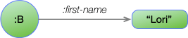
This is represented with the statement:
:B :first-name "Lori"
A group of statements like this provides the complete description for a graph. Using this we can represent the entire Organization Chart from above with the following statements:
| Graph Statements |
|---|
| :A :first-name "Sally" |
| :A :last-name "Smith" |
| :A :title "CEO" |
| :B :reports-to :A |
| :B :first-name "Lori" |
| :B :last-name "Luck" |
| :B :title "CTO" |
| :C :reports-to :B |
| :C :first-name "Carly" |
| :C :last-name "Cool" |
| :C :title "Engineering Manager" |
| :D :reports-to :C |
| :D :first-name "Jenny" |
| :D :last-name "James" |
| :D :title "QA Engineer" |
| :E :reports-to :C |
| :E :first-name "Mary" |
| :E :last-name "Mercy" |
| :E :title "Engineer" |
If we use this information to build a picture, we can reconstruct the original graph image or something very close. Remember that it doesn't matter how a graph image is laid out, so long as it has all of the correct nodes and edges.
The information here is very dense, but it is ideal for computers. It also follows a simple pattern that we can use when accessing the data.
When we want to access data in a graph, we use an approach called a pattern.
A graph pattern looks like a triple, but with one or more of the elements not filled in. It acts as a template that matches any triples with matching elements. For now, we will mark the empty elements with an underscore character: _
For instance, this pattern will match all triples that describe a :first-name:
[ _ :first-name _ ]
If we compare this to the graph with the organization chart, this will match the following statements from the graph (remembering that statements are triples):

| Graph Statements |
|---|
| :A :first-name "Sally" |
| :B :first-name "Lori" |
| :C :first-name "Carly" |
| :D :first-name "Jenny" |
| :E :first-name "Mary" |
Finding which statements in a graph will match a pattern is called Resolving the pattern.
Now that we have matched a pattern to triples, we want to see what was in them. To get this information, we can attach a variable to the blank spaces. When the pattern matches a triple then the variable in a position will be set to the value in that position.
Let's look at a pattern with just one space. This pattern looks for the :first-name of node :E.
[ :E :first-name _ ]
When this pattern is applied to the graph it matches just a single statement in the graph. We can see the relevant part of the graph here:

:E :first-name "Mary"
The blank space in this pattern can be replaced by a variable so that we can access the data that was found. Variables are represented as a name with a ? character at the front. We can re-write the pattern to use the variable ?n in the blank space:
[ :E :first-name ?n ]
So when this pattern is resolved against the graph the variable ?n will be made equal to "Mary".
Most of the time a pattern will have multiple statements that it will match. In this case, the match will be a series of values for the variables in the pattern. To see this, let's look for all of the :first-name elements again. This time, we will name both the first and last node positions with the variables ?node and ?n:
[?node :first-name ?n]
This matches the statements we saw earlier:
:A   :first-name   "Sally"
:B   :first-name   "Lori"
:C   :first-name   "Carly"
:D   :first-name   "Jenny"
:E   :first-name   "Mary"
But because we have now attached variables to the blank parts of the pattern, the result leads to a series of values for ?node and ?n:
?node = :A    ?n = "Sally"
?node = :B    ?n = "Lori"
?node = :C    ?n = "Carly"
?node = :D    ?n = "Jenny"
?node = :E    ?n = "Mary"
The variables in each of these values are connected to each other, so when ?node is :A then ?n is "Sally", and when ?node is :B then ?n is "Lori". We call each of these variable/value groups a binding. Within a binding, each variable is bound.
So in the first binding the ?node is bound to :A and the ?n is bound to "Sally". In the last binding the ?node is bound to :E and the ?n is bound to "Mary".
The result of matching a pattern to a graph is a set of bindings. In this case, the set of bindings is 5 long.
In fact, whenever a pattern returns only a single result, like in the previous section, it will also be a set of bindings. But as we saw, that set was only one binding long.
Using what we have seen so far, we can try to answer the question, "Is 'James' a first name or a last name?"
- We know that :first-name and :last-name refer to strings like "James" that will appear at the end of a pattern. So the pattern should end with "James".
- We know that :first-name and :last-name are edge names, and edge names appear in the middle of a pattern. We don't know which one we're going to get, so we will need a variable to put here. That variable will get the answer.
- We don't know which nodes will appear at the start of the statements. So we will need a variable at the start. However, we don't care what these values are. We can name it something like
?node, or we can just leave it unnamed with_.
This gives us the following pattern:
[ _ ?edge "James" ]
When this pattern is applied to the graph, it will match the single statement in the graph:
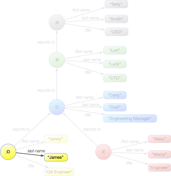
:D :last-name "James"
So the result is this single binding:
?edge = :last-name
A Join is the process of connecting multiple patterns to answer a more complex question of a graph.
For instance, say we want to know what Jenny's title is. If we look at the relevant section of the graph, we can see that this information is available from 2 statements:
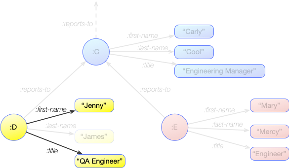
:D   :first-name   "Jenny"
:D   :title        "QA Engineer"
Consider what we need here:
- A statement where a node has :first-name of "Jenny"
- A statement where a node has a :title
The pattern for the first part is:
[ ?node :first-name "Jenny" ]
This will lead to the statement:
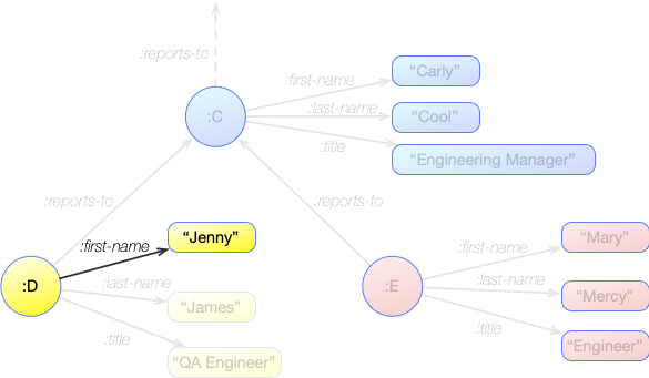
:D :first-name "Jenny"
This gives us the single binding:
?node |
|---|
| :D |
The pattern for the second part is:
[ ?node :title ?title ]
This pattern resolves to these statements:

:A   :title        "CEO"
:B   :title        "CTO"
:C   :title        "Engineering Manager"
:D   :title        "QA Engineer"
:E   :title        "Engineer"
This gives us these variable bindings:
?node |
?title |
|---|---|
| :A | "CEO" |
| :B | "CTO" |
| :C | "Engineering Manager" |
| :D | "QA Engineer" |
| :E | "Engineer" |
The resolution of the first pattern was what we were looking for, but the resolution of the second pattern gives us much more than we want. Instead, we just want the title statements for the node that we found with the pattern that looked for :first-name.
This is where we can use a Join operation. If two patterns share a variable, then a join will return just those results where the variables match. If the value of a binding only appears on one side of a join, then it gets discarded.
Both of our patterns use a ?node variable, so we can join these results just by writing the patterns together:
[ ?node :first-name "Jenny" ] [ ?node :title ?title ]
?node (pattern 1) |
?node (pattern 2) |
?title (pattern 2) |
|---|---|---|
| :D | :D | "QA Engineer" |
The final result is a single binding:
?node |
?title |
|---|---|
| :D | "QA Engineer" |
The answer that we are looking for is in the binding for ?title. The ?node value is not needed here
By having a variable representing nodes in the graph, multiple joins can be used to step from one node to another.
Let's try answering the question, "What is the title of the person the Engineer reports to?"
- First, find the node representing the person with the title "Engineer".
- Then find the person they report to.
- Get the title of this person.
We can get the node representing the engineer, and bind that to the variable ?engineer:
[ ?engineer :title "Engineer" ]
This resolves to find:
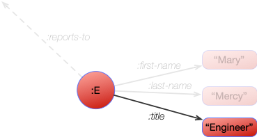
Which returns a single binding of:
?engineer |
|---|
| :E |
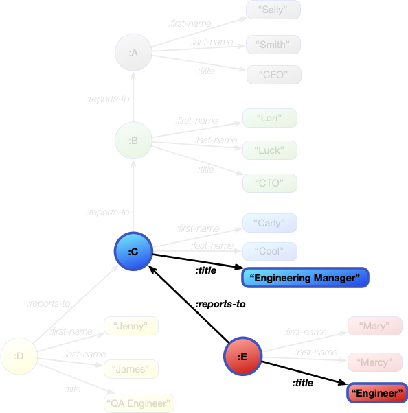
The next step is to find the person that ?engineer reports to. We will bind that to ?manager:
[ ?engineer :reports-to ?manager ]
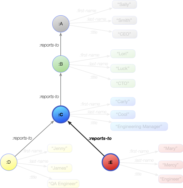
This image shows all the :reports-to statements in the graph, but because the ?engineer is currently bound to a single value of :E then only a single statement will match the join. This is shown in bold in the graph image above.
?engineer (pattern 1) |
?engineer (pattern 2) |
?manager (pattern 2) |
|---|---|---|
| :E | :E | :C |
So the bindings after this first join are:
?engineer |
?manager |
|---|---|
| :E | :C |
Finally, we can get the title of the ?manager:
[ ?manager :title ?title ]
We see here all the :title statements in the graph, but again, the ?manager variable has a single binding of :C. The resulting statement is shown in bold, and this is the only binding that gets through:
?engineer |
?manager (pattern 2) |
?manager (pattern 3) |
?title (pattern 3) |
|---|---|---|---|
| :E | :C | :C | "Engineering Manager" |
The bindings after this second join are:
?engineer |
?manager |
?title |
|---|---|---|
| :E | :C | "Engineering Manager" |
The final expression contains all three of these patterns joined to select the required part of the graph.
[ ?engineer :title "Engineer" ] [ ?engineer :reports-to ?manager ] [ ?manager :title ?title ]
This image of the graph shows where the joined patterns matched.
These patterns gave us the final bindings of the joins:
?engineer |
?manager |
?title |
|---|---|---|
| :E | :C | "Engineering Manager" |
Inspecting the value of the ?title variable provides the answer.
To find data in a graph, we perform a Query. This is basically everything we have looked at so far, along with a description of the variables that we want to read.
The basic structure for a simple query in Asami is:
[:find variables :where patterns]
The patterns are simply the patterns already discussed. Adding more patterns leads to more joins between the patterns. The variables describe which of the bound variables we are interested in. The whole thing appears as a vector.
For instance, in the last section we developed an expression of graph patterns that will find the title of the person the engineer reports to. The query for this would be:
[:find ?title :where [?engineer :title "Engineer"] [?engineer :reports-to ?manager] [?manager :title ?title]]
This has placed the patterns as the :where clause, and the required ?title as the desired output in the :find clause.
The ?engineer and ?manager variables can also appear in the :find clause, but they are not needed, so they have been left out.
The asami.core namespace contains the functions needed to access a graph. After establishing a connection to a database, the database value can be retrieved with the function asami.core/db. This is then provided along with a query as the parameters for the querying function asami.core/q. For instance, to execute the previous query on an existing connection to a database:
(def database (asami.core/db connection))
(def result (asami.core/q '[:find ?title
                            :where [?engineer :title "Engineer"]
                                   [?engineer :reports-to ?manager]
[?manager :title ?title]] database)Some other examples of simple queries:
- Get a list of all the titles
[:find ?title :where [_ :title ?title]]
?title |
|---|
| "CEO" |
| "CTO" |
| "Engineering Manager" |
| "QA Engineer" |
| "Engineer" |
- Get the full names of all the people
[:find ?fname ?lname :where [?person :first-name ?fname] [?person :last-name ?lname]]
?fname |
?lname |
|---|---|
| "Sally" | "Smith" |
| "Lori" | "Luck" |
| "Carly" | "Cool" |
| "Jenny" | "James" |
| "Mary" | "Mercy" |
- Get the first names of the people who report to the Engineering Manager
[:find ?name :where [?manager :title "Engineering Manager"] [?person :reports-to ?manager] [?person :first-name ?name]]
?name |
|---|
| "Jenny" |
| "Mary" |
Hopefully, this will have provided you with an understanding of graph structures and patterns for querying them. There are more operations available in queries, but these are all refinements on what has been shown here.
Some examples of more advanced operations in queries are:
- Filtering
- Bindings
- Parameter passing
- Disjunctions
- Negations
- Aggregation
- Aggregate Grouping
- Transitive properties
- Subquerying
Queries can also be provided as maps of clause names to their values, rather than vectors.
This will all be covered in other pages. However, in many real-world cases queries only require simple patterns and joins.