Tutorials
- Introduction
- Metagenomic pathogen detection
- Contig taxonomic assignment and auxiliary modules
- Writing large scale sequence analysis workflows

Your new friends! MMseqs2 ultra fast and sensitive protein search, Linclust clustering huge protein sequence sets in linear time and Plass Protein-level assembly to increases protein sequence recovery from complex metagenomes.
Here you will learn the basic usage of MMseqs2 as well as expert tricks to take advantage of the ability of chaining different MMseqs2 modules to produce custom workflows.
We will use Conda to setup all required software for this tutorial. If you haven't setup Conda yet, please do so first and then execute:
conda create -n tutorial -c conda-forge -c bioconda mmseqs2 plass megahit prodigal hmmer sra-tools
conda activate tutorial
The generic syntax for mmseqs and plass calls is always the
following:
mmseqs <command> <db1> [<db2> ...] --flag --parameter 42
The help text of mmseqs shows, by default, only the most important
parameters and modules. To see a full list of parameters and modules use
the -h flag.
If you are using Bash as your shell, you can activate tab-auto-completion of commands and parameters:
source $CONDA_PREFIX/util/bash-completion.sh
A 61-year-old man was admitted in December 2016 with bilateral headache, gait instability, lethargy, and confusion. Because of multiple tick bites in the preceding 2 weeks, he was prescribed the antibiotic doxycycline for presumed Lyme disease. Over the next 48 hours, he developed worsening confusion, weakness, and ataxia. He returned to the referring hospital and was admitted. He lived in a heavily wooded area in New Hampshire, had frequent tick exposures, and worked as a construction contractor in basements with uncertain rodent and bat exposures. His symptoms were diagnosed as Encephalitis and the causative agent --- not known.
- Your task will be to identify the pathogenic root cause of the disease.
This pathogen is usually confirmed by a screening antibody test, followed by a plaque reduction neutralization test. However, this takes 5 weeks, which was too slow to affect the patient's care. As traditional tests done in the first week of the patient's hospital stay did not reveal any conclusive disease cause, the doctors were running out of options. Therefore a novel metagenomic analysis was performed.
Metagenomic sequencing from cerebrospinal fluid was performed on hospital day 8. It returned 14 million short nucleotide sequences (reads).
The authors of the study removed all human reads using Kraken (Wood and Salzberg 2014) and released a much smaller set of 226,908 reads on the SRA (https://trace.ncbi.nlm.nih.gov/Traces/sra/sra.cgi). Kraken extracts short nucleotide subsequences of length k, also called k-mers, and compares them to a reference database where k-mers point to taxonomic labels. In case of exact matching it is able to assign taxonomy.
- Why didn't the authors release the complete dataset?
- Demanding exact k-mer matching in Kraken has benefits for removing human reads. Why?
- What is the SRA? How many samples are there in the SRA currently? How many bases are publicly available on the SRA in total?
We will use the sequence search tool MMseqs2 (Steinegger and Soeding 2017) to find the cause of this patient's disease. MMseqs2 translates the nucleotide reads to putative protein fragments, searches against a protein reference database and assigns taxonomic labels based on the found reference database hits.
- Why might a protein-protein search be useful for finding bacterial or viral pathogens? How does this compare with Kraken's approach?
To not spoil the mystery too early, we prepared a FASTA file containing the reads. Download this file first:
wget http://wwwuser.gwdg.de/~compbiol/mmseqs2/tutorials/mystery_reads.fasta
The sequencing machine returns paired-end reads where sequencing starts in opposite directions from two close-by points to cover the same genomic region. Some of these paired reads overlap enough to be merged into a single read with FLASH (Magoc and Salzberg 2011).
We will also need a reference database of proteins. For this we will use the Swiss-Prot which is the manually curated, high-quality part of the Uniprot (UniProt Consortium 2014) protein reference database. We are using this smaller subset of about 500,000 proteins, since the full Uniprot with over 175,000,000 sequences requires too many computational resources. Each protein in Uniprot has a taxonomic label. Let us prepare this database:
# Download the database
wget http://wwwuser.gwdg.de/~compbiol/mmseqs2/tutorials/uniprot_sprot_2018_03.fasta.gz
wget http://wwwuser.gwdg.de/~compbiol/mmseqs2/tutorials/uniprot_sprot_2018_03_mapping.tsv.gz
gunzip uniprot_sprot_2018_03_mapping.tsv.gz

# Create a taxonomically annotated sequence database
mmseqs createdb uniprot_sprot_2018_03.fasta.gz uniprot_sprot
mmseqs createtaxdb uniprot_sprot tmp --tax-mapping-file uniprot_sprot_2018_03_mapping.tsv
Through a similarity search we will transfer the annotation of the reference protein to our unknown reads.
mmseqs createdb mystery_reads.fasta reads
mmseqs taxonomy reads uniprot_sprot lca_result tmp -s 2
MMseqs2 will create a result database in your current working directory.
This database consists of files, whose names start with lca_result. We
can convert this database into a human readable tab separated values
file (TSV), a common format in bioinformatics:
mmseqs createtsv reads lca_result lca.tsv
In this file you see for every read a numeric taxonomic identifier, a
taxonomic rank and a taxonomic label. However, due to the large number
of reads, it is hard to gain insight by skimming the file. MMseqs2
offers a module to summarize the data into a single file report.txt:
mmseqs taxonomyreport uniprot_sprot lca_result report.txt
- What is the most common species in this dataset?
- Why are there so many different eukaryotic sequences? Were they really in the spinal fluid sample?
MMseqs2 can also generate an interactive visualization of the data using Krona (Ondov, Bergman, and Phillippy 2011). Adapt the previous call to generate a Krona report:
mmseqs taxonomyreport uniprot_sprot lca_result report.html --report-mode 1
This generates a HTML file that can be opened in a browser. This
offers an interactive circular visualization where you can click on each
label to zoom into different parts of the hierarchy.
Look up the following encephalitis causing agents in Wikipedia.
-
Borrelia bacterium
-
Herpes simplex virus
-
Powassan virus
-
West Nile virus
-
Mycoplasma
-
Angiostrongylus cantonensis
- Based on the literature, which one is the most likely pathogen?
- For which species do you find evidence in the metagenomic reads?
- Approximately how many reads belong to the pathogen? Based on this number, how would you determine if it is significant evidence for an actual presence of this agent?
We now want to take a closer look only at the reads of the pathogen. To filter the result database, we will need the pathogen's numeric taxonomic identifier. Use the NCBI Taxonomy Browser to find it, by searching for its name.
- What is the taxon identifier of the pathogen? Did you find one or more?
Now we can call a different MMseqs2 module to retrieve only the reads that belong to this pathogen. Replace XXX with the number(s) you just found. If you found multiple, concatenate them with a comma character.
mmseqs filtertaxdb uniprot_sprot lca_result lca_only_pathogen --taxon-list XXX
We now get a list of all queries that were filtered out, meaning they were annotated as pathogenic.
grep -Pv '\t1$' lca_only_pathogen.index > pathogenic_read_ids
With a few more commands we can convert our taxonomic labels back into a FASTA file:
mmseqs createsubdb pathogenic_read_ids reads reads_pathogen

mmseqs convert2fasta reads_pathogen reads_pathogen.fasta
- How many reads of the pathogen are in this resulting FASTA file?
We want to try to recover the protein sequences of the pathogen.
- Which proteins do you expect to find in the pathogen you discovered? Search the internet.
We will use the protein assembly method Plass (Steinegger, Mirdita, and Söding 2019) to find overlapping reads and generate whole proteins out of the best matching ones.
plass assemble reads_pathogen.fasta pathogen_assembly.fasta tmp
Take a look at the generated FASTA file pathogen_assembly.fasta.
- How many sequences were assembled?
- Do some of the sequences look similar to each other?
Plass will uncover a lot of variation in the reads and output many similar proteins. We can use the sequence clustering module in MMseqs2 to get only representative sequences.
mmseqs easy-cluster pathogen_assembly.fasta assembly_clustered tmp
You will see three files starting with assembly_clustered:
-
assembly_clustered_all_seqs.fasta -
assembly_clustered_cluster.tsv -
assembly_clustered_rep_seq.fasta
Take a look at the last one assembly_clustered_rep_seq.fasta. This
file contains all representative sequences, meaning the sequence that
the algorithm chose as the most representative within this cluster.
- How many sequences remain now?
- How well does this agree with what you expected according to your internet search?
We will look for known protein domains to identify the proteins we found. Instead of the MMseqs2 command line, we use the MMseqs2 webserver, which will visualize the results. Paste the content of the FASTA file containing the representative sequences into the webserver and make sure to select all three target databases (PFAM, PDB, Uniclust): https://search.mmseqs.com
- Which of the expected proteins do you find?
Despite being able to identify the causative agent. The pathogen is very hard to treat. The patient had minimal neurological recovery and was discharged to an acute care facility on hospital day 30. Seven months after discharge, he was reportedly able to nod his head to questions and slightly move his upper extremities and toes.
You can find the publication about this patient and dataset here (Piantadosi et al. 2018). Please look at it only after trying to answer the questions yourself.
UniProt Consortium. 2014. "UniProt: A Hub for Protein Information." Nucleic Acids Research 43 (D1): D204--D212.
Magoc, Tanja, and Steven L. Salzberg. 2011. "FLASH: Fast Length Adjustment of Short Reads to Improve Genome Assemblies." Bioinformatics 27 (21): 2957--63.
Ondov, Brian D, Nicholas H Bergman, and Adam M Phillippy. 2011. "Interactive metagenomic visualization in a Web browser." BMC Bioinformatics 12 (1): 385.
Piantadosi, Anne, Sanjat Kanjilal, Vijay Ganesh, Arjun Khanna, Emily P Hyle, Jonathan Rosand, Tyler Bold, et al. 2018. "Rapid Detection of Powassan Virus in a Patient With Encephalitis by Metagenomic Sequencing." Clinical Infectious Diseases 66 (5): 789--92.
Steinegger, Martin, Milot Mirdita, and Johannes Söding. 2019. "Protein-level assembly increases protein sequence recovery from metagenomic samples manyfold." Nature Methods 16 (7): 603--6.
Steinegger, Martin, and Johannes Soeding. 2017. "MMseqs2: Sensitive Protein Sequence Searching for the Analysis of Massive Data Sets." bioRxiv, 079681.
Wood, Derrick E, and Steven L Salzberg. 2014. "Kraken: ultrafast metagenomic sequence classification using exact alignments." Genome Biology 15 (3): R46.
Download an example input contig and create a MMseqs2 database:
wget https://raw.githubusercontent.com/soedinglab/metaeuk-regression/205bc3f26bfa335366e2f00dccbc6900306cd4a8/sacc_tax/NC_001133.9_100425_153163.fa .

ls
# NC_001133.9_100425_153163.fa
Use createdb with the input contig file to create a MMseqs2 database:
mmseqs createdb NC_001133.9_100425_153163.fa contig
If you wish to examine the 19 annotated proteins coded on this contig, you can download them too (they won't be used in the tutorial):
wget https://raw.githubusercontent.com/soedinglab/metaeuk-regression/205bc3f26bfa335366e2f00dccbc6900306cd4a8/sacc_tax/sacc_prots_in_segment.fa .
mmseqs databases allows downloading various sequences databases and any accompanying taxonomic information (full details). We will use this command to download SwissProt:
mmseqs databases UniProtKB/Swiss-Prot swissprot tmp
As you can see by examining the files with the swissprot prefix, the downloaded database is an MMseqs2 seqTaxDb (read more about the format).
The following command runs the 4-step contig taxonomy workflow. It extracts protein fragments in six frames and searches them against SwissProt using the accelerate 2bLCA method (--lca-mode 3). It then conducts a vote among all assigned fragments, selecting the most specific taxonomic label, which has at least 50% support (--majority 0.5) of the -log(E-value) weights (--vote-mode 1). The parameter --tax-lineage 2 indicates the output will include the full lineage information as NCBI taxids.
mmseqs taxonomy contig swissprot assignments tmpFolder --tax-lineage 2 --majority 0.5 --vote-mode 1 --lca-mode 3 --orf-filter 1
The raw assignments database can be converted to a tab separated (tsv) file.
mmseqs createtsv contig assignments assignRes.tsv
Let's take a closer look at the assignment:
cat assignRes.tsv
# NC_001133.9     4932    species Saccharomyces cerevisiae        32      32      30      0.890   131567;2759;33154;4751;451864;4890;716545;147537;4891;4892;4893;4930;4932
The contig has been assigned at the species level to taxid 4932 (Saccharomyces cerevisiae). The assignment is based on 32 protein fragments, which passed the fast prefilter selection (step II of the TaxPerContig algorithm). Of these, all 32 fragments received a label and of these, 30 agree with the label assigned to the contig (i.e., they were assigned to species 4932 or to a strain below it). The fraction of -log(E-value) support of the label is 89%.
This visualization can be created for the contigs assignments as well as for the fragment assignments to see the distribution of labels among them. To create a Krona (--report-mode 1) visualization for the fragments:
mmseqs taxonomyreport swissprot tmpFolder/latest/orfs_tax fragmentsReport.html --report-mode 1
To create a Kraken report (--report-mode 0) for the contig:
mmseqs taxonomyreport swissprot assignRes contigReport.txt --report-mode 0
The MMseqs2 Wiki provides further information about other taxonomic modules in MMseqs2 (e.g., creating subdbs of a seqTaxDb) and the various parameter values (e.g., controlling the LCA modes).
We will show on a human gut metagenomic dataset (SRA run ERR1384114)
what the advantages of using Linclust
(linear time clustering algorithm, (Steinegger and Söding 2018)), Plass
(Protein Level Assembly, (Steinegger, Mirdita, and Söding 2018)) and
MMseqs2 are over the more conventional pipeline with MegaHit(Li et al.
2015), Prodigal (Hyatt et al. 2010) and HMMER (Eddy 2009).
We use Plass to assemble a catalogue of protein sequences directly from the reads, without the nucleic assembly step. It recovers 2 to 10 times more protein sequences from complex metagenomes than other state-of-the-art methods and can assemble huge datasets.
First we will load the dataset from the SRA with sra-tools:
prefetch ERR1384114
fasterq-dump ERR1384114
Alternatively, the reads can be downloaded directly from the European Nucleotide Archives's download server:
wget https://ftp.sra.ebi.ac.uk/vol1/fastq/ERR138/004/ERR1384114/ERR1384114_1.fastq.gz
wget https://ftp.sra.ebi.ac.uk/vol1/fastq/ERR138/004/ERR1384114/ERR1384114_2.fastq.gz
gunzip ERR1384114_1.fastq.gz
gunzip ERR1384114_2.fastq.gz
The standard genomic assemblies prevent many reads to assemble due to low coverage and micro-diversity. To run this protein-level assembly, use the command
plass assemble ERR1384114_1.fastq ERR1384114_2.fastq plass_proteins.fasta tmp
or type plass assemble -h to see all available options.
As a matter of comparison, run the usual pipeline using MegaHit for genomic assembly:
megahit -1 ERR1384114_1.fastq -2 ERR1384114_2.fastq -o megahit_assembly
Then extract proteins using Prodigal in metagenomics mode:
prodigal -i megahit_assembly/final.contigs.fa -a prodigal_proteins.fasta -p meta
Take a look at the FASTA files produced by Plass and Prodigal. To check
the number of detected proteins, you can count the number of FASTA
headers (lines beginning with the > character):
grep -c "^>" file.faa
Since Plass assembles with replacement of reads, the catalogue will
contain some redundancy. You can reduce this catalogue by clustering it,
for instance, to 90% of sequence identity, and asking for the
representative sequence that cover at least 95% of the members. For
this, you can either use the easy-cluster (sensitive clustering) or
easy-linclust (linear time fast clustering) modules of MMseqs2:
mmseqs easy-cluster plass_proteins.fasta clustered_proteins tmp --min-seq-id 0.9 -c 0.95 --cov-mode 1
Both the default MMseqs2 clustering and Linclust link two sequences by an edge based on three local alignment criteria:
-
a maximum E-value threshold (option
-e, default 10^-3) computed according to the gap-corrected Karlin-Altschul statistics; -
a minimum coverage (option
-c, which is defined by the number of aligned residue pairs divided by either the maximum of the length of query/centre and target/non-centre sequences alnRes/max(qLen,tLen) (default mode,--cov-mode0), by the length of the target/non-centre sequence alnRes/tLen (--cov-mode1), or by the length of the query/centre alnRes/qLen (--cov-mode 2); -
a minimum sequence identity (
--min-seq-id) with option--alignment-modedefined as the number of identical aligned residues divided by the number of aligned columns including internal gap columns, or, by default, defined by a highly correlated measure, the equivalent similarity score of the local alignment (including gap penalties) divided by the maximum of the lengths of the two locally aligned sequence segments. The score per residue equivalent to a certain sequence identity is obtained by a linear regression using thousands of local alignments as training set.
You can count the number of cluster representatives in the FASTA file
clustered_proteins_rep_seq.fasta again using the previous grep command.
The previous easy-cluster command is a shorthand to deal directly with
FASTA files as input and output. However, MMseqs2's modules do not
use the FASTA format internally. Since the goal of this tutorial is to
make you an expert in using MMseqs2 workflows, we will explain and use
the MMseqs2 database formats and create FASTA files only for downstream
tools.
You can convert a FASTA file to the MMseqs2 database format using:
mmseqs createdb plass_proteins.fasta plass_proteins_db
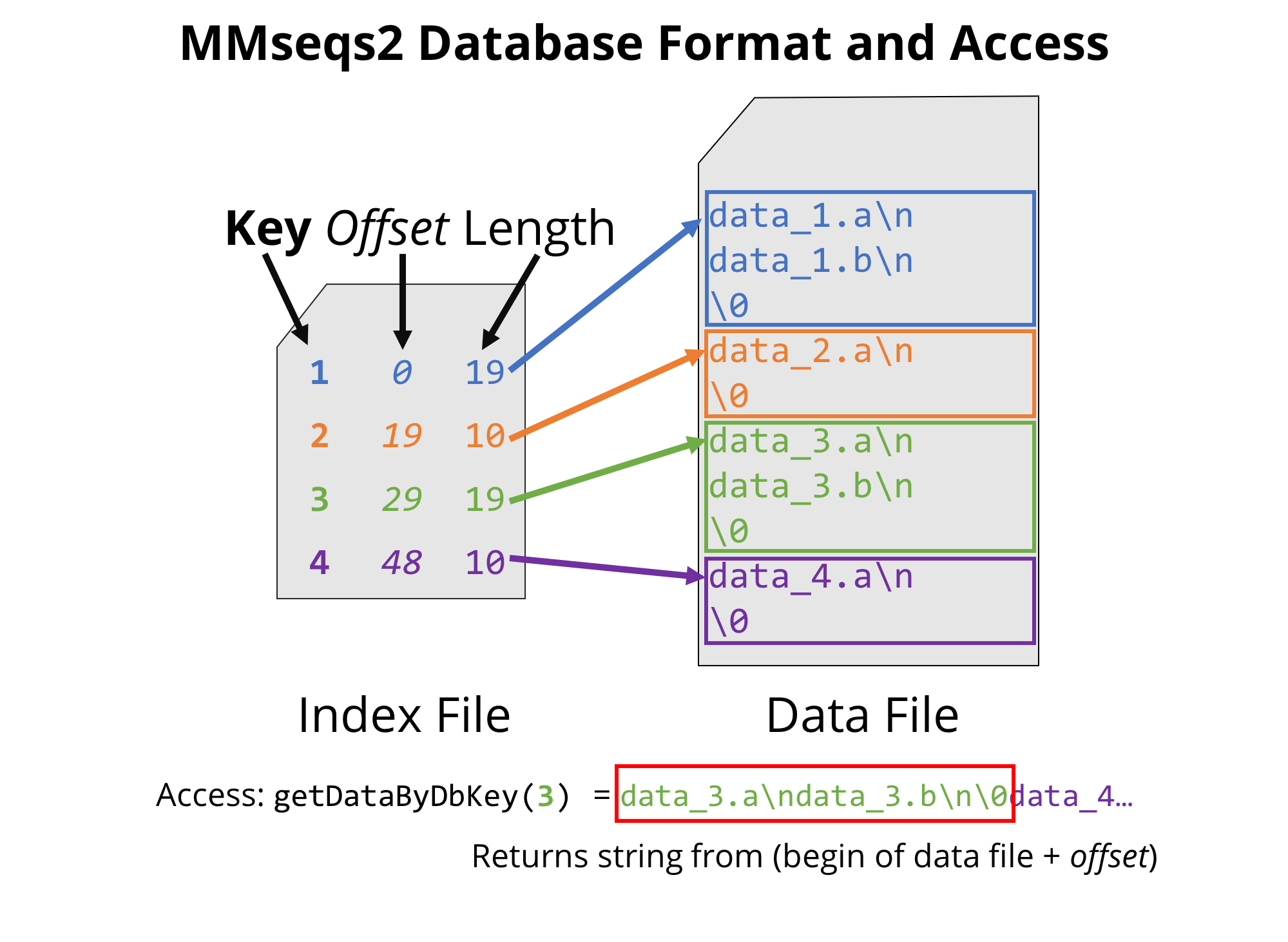
This generates several files: a data file plass_proteins_db together
with an index file plass_proteins_db.index. The first file contains
all the sequences separated by a null byte \0. We coin more generally
any data record an entry, and each entry is associated with a unique
key (integer number) that is stored in the index file.
MMseqs2 database format, through which all MMseqs2 modules can be easily and efficiently chained.
The corresponding headers are stored in a separate database with a _h
suffix (plass_proteins_db_h).
The .dbtype file helps to keep track of the database type (amino-acid,
nucleic, profile, etc.).
The .lookup file is a lookup file linking the keys to their sequence
accession as specified in their FASTA header.
The format of this index file is tab-separated and reports one line per entry in the database, specifying a unique key (column 1), the offset and the length of the corresponding data (columns 2 and 3 respectively). As we will make use of the efficient structure later on in the tutorial, you can already take a look at the index file structure with:
head plass_proteins_db.index
Let's re-run the clustering of the catalogue database with our fresh database:
mmseqs cluster plass_proteins_db plass_proteins_db_clu tmp --min-seq-id 0.9 -c 0.95 --cov-mode 1
This creates a cluster database where each entry has the key of its representative sequence, and whose data consists of the list of keys of its members:
# the index file contains entries whose
# keys are of those of their representative sequence
head plass_proteins_db_clu.index

# you will see the keys belonging to different clusters
# (one per line) and such that every cluster is
# separated by a null byte shown as ^@ in less
less plass_proteins_db_clu.0
Note: This is a general principle in MMseqs2: the keys are always consistent between databases (input and output, clustering and sequence databases, and potentially intermediate files.
Therefore, to count the number of clusters, you can count the number of lines in the index file using:
wc -l plass_proteins_db_clu.index
To get domain annotation for your protein catalogue, we search the sequences against a database of Pfam profiles.
To do this, we have to setup this profile database first:
# Download the latest Pfam from EBI servers
wget http://ftp.ebi.ac.uk/pub/databases/Pfam/current_release/Pfam-A.full.gz

# Convert Pfam stockholm format to an aligned FASTA database
mmseqs convertmsa Pfam-A.full.gz pfam_msa

# Convert to our MMseqs2 internal profile format
mmseqs msa2profile pfam_msa pfam_profile --match-mode 1 --msa-type 2
Now we can annotate our sequences against this database:
# first create a sequence database of the representative sequences
mmseqs createsubdb plass_proteins_db_clu.index plass_proteins_db  plass_proteins_rep

# -s 7 for high sensitivity
mmseqs search plass_proteins_rep pfam_profile mmseqs_result_pfam tmp -s 7

# you can make it human-readable in TSV format
mmseqs createtsv plass_proteins_rep pfam_profile mmseqs_result_pfam mmseqs_result_pfam.tsv

# and also return a FASTA file of representatives
mmseqs convert2fasta plass_proteins_rep plass_proteins_rep.fasta
You can post-process the annotation file to retrieve only annotations of high confidence:
# check that the e-values are shown in column 4 of the search result database
head mmseqs_result_pfam.0

# create a new database containing
# only annotations of e-value <= 1e-5
mmseqs filterdb mmseqs_result_pfam strong_pfam_annotations \
    --filter-column 4 --comparison-operator le --comparison-value 1e-5
An advanced way to extract the entries that did not get a reliable annotation uses the fact that if no hit was found for a given sequence, the corresponding entry in the data file will be empty, resulting in a data length of 1 (for the null byte) in the index file:
# extract the keys of entries having no annotation better than 1e-5
awk '$3==1 {print $1}' strong_pfam_annotations.index > uncertain_function_keys

# create a FASTA file for further investigation in downstream tools (HHblits for instance)
# First extract sub-database containing the protein sequences of uncertain function
mmseqs createsubdb uncertain_function_keys plass_proteins_rep plass_proteins_uncertain

# convert it to a fasta file
mmseqs convert2fasta plass_proteins_uncertain plass_proteins_uncertain.fasta
You can compare (time and number of annotation) with HMMER3. However, we have to again create the database first:
hmmbuild pfam_hmmer Pfam-A.full.gz
hmmpress pfam_hmmer

time hmmscan --notextw --noali --tblout "hmmer.tblout" \
    --domtblout "hmmer.domtblout" pfam_hmmer plass_proteins_rep.fasta

# check the number of annotated proteins
#   for MMseqs2
awk '$3 > 1 {print $1}' mmseqs_result_pfam.index | wc -l
#   for HMMER
tail -n+4 hmmer.tblout | cut -c 21-30 | sort -u | wc -l
We will take advantage of MMseqs2's modular architecture to create a workflow (bash script) that calls MMseqs2 tools to deeply cluster a set of proteins.
Let's first create a cascaded clustering workflow: after a first clustering step, the representative sequences of each of the clusters are searched against each other and the result of the search is again clustered. By repeating this procedure iteratively, one gets a deeper clustering of the original set.
Try to code complete the following script:
#!/bin/bash -e

MAX_STEPS="3"
INPUT="plass_proteins_db"
for step in $(seq 1 ${MAX_STEPS}); do
    # we do not use the cluster mmseqs command as it
    # already is a cascaded workflow clustering
    mmseqs search "$INPUT" "$INPUT" search_step_${step} tmp
    mmseqs clust "$INPUT" search_step_${step} clu_step_$step
    mmseqs result2repseq ...
    inputdb=...
done

# Then merge the clustering steps
mmseqs mergeclusters plass_proteins_db deep_cluster_db ...
Try your script with 3 steps, and check the clustering depth (number of clusters) at each step:
wc -l clu_step_*.index
What do you notice?
To make a deeper clustering of your protein set, one idea is to create a
cascaded clustering where the sequence search at every iteration is
replaced by a profile to sequence search (more sensitive search than
sequence to sequence searches). Write your own workflow that will be
using the result2profile module. After adjusting your workflow to
handle profiles also add the –add-self-matches parameter to the search
to assure that the query is contained in each search results.
Did you manage to cluster more deeply?
You can get the distribution of your cluster sizes by calling:
# get the size of every cluster
mmseqs result2stats plass_proteins_db plass_proteins_db \
    deep_cluster_db deep_cluster_sizes --stat linecount

# show the distribution, here we want to first get rid of all null bytes with tr
tr -d '\0' < deep_cluster_sizes | sort -n | uniq -c
Compare this clustering to your first cascaded clustering.
Let's check the most abundant genes in our dataset. To this end, we want to map the ORFs from the reads to the protein catalogue, and count the number of hits on each of the proteins.
Write an MMseqs2 workflow that:
-
creates a read sequence database from the FASTA files (
createdb) -
extracts the ORFs from the read database (
extractorfs), -
translate the nucleotide ORFs to protein sequences (
translatenucs), -
map them on the proteins (
prefilterwith option-s 2since mapping calls for high sequence identity), -
score the prefilter hits with a gapless alignment (
rescorediagonalwith options-c 1 –cov-mode 2 –min-seq-id 0.95 –rescore-mode 2 -e 0.000001 –sort-results 1to have significant hits and fully covered by the protein sequence), -
keep the best mapping target (
filterdbwith flag–extract-lines 1), -
in the database output from the last step, every entry is a read-ORF. Now you should transpose the database so that each contig is an entry, and the data is the list of mapped read-ORFs (
swapresults), -
count the number of mapped read-ORF (
result2stats). Advanced: instead of just count the reads, sum up the aligned length and divide it by the contig lengthapplyandawk. The contig length and alignment length (alnEnd - alnStart) is in the alignment format.
We can use createtsv to output the abundances as a TSV formatted file:
# Create a flat file
mmseqs createtsv plassProteinsReduced plassProteinsReduced\
    mapAbundances mapAbundances.tsv --target-column 0
Based on the explanation of the Linclust algorithm, try to code its workflow using:
-
kmermatcher -
rescorediagonal -
clust
Take a look at the real Linclust workflow.
This version is slightly more involved as it integrates a redundancy
reduction step (the pre_clust prefiltering by high Hamming distance),
and uses a trick using filterdb with the flag –filter-file to apply
the workflow you just built only on the non-redundant entries. At
the end of the file, you can also spot a merging step to recover the
redundant part in the final clustering.
We hope that you are more familiar with the MMseqs2 environment, and that you enjoy its modularity and flexibility for creating new workflows. Due to time and virtual machine constraints we chose a rather small metagenomic dataset, but using MMseqs2 on bigger datasets should convince you of its scalability.
Eddy, Sean R. 2009. "A New Generation of Homology Search Tools Based on Probabilistic Inference." In Genome Informatics 2009: Genome Informatics Series Vol. 23, 205--11. World Scientific.
Hyatt, Doug, Gwo-Liang Chen, Philip F LoCascio, Miriam L Land, Frank W Larimer, and Loren J Hauser. 2010. "Prodigal: Prokaryotic Gene Recognition and Translation Initiation Site Identification." BMC Bioinformatics 11 (1): 119.
Li, Dinghua, Chi-Man Liu, Ruibang Luo, Kunihiko Sadakane, and Tak-Wah Lam. 2015. "MEGAHIT: An Ultra-Fast Single-Node Solution for Large and Complex Metagenomics Assembly via Succinct de Bruijn Graph." Bioinformatics 31 (10): 1674--6.
Steinegger, Martin, Milot Mirdita, and Johannes Söding. 2019. "Protein-Level Assembly Increases Protein Sequence Recovery from Metagenomic Samples Manyfold." Nature Methods 16 (7) 603-609.
Steinegger, Martin, and Johannes Söding. 2017. "MMseqs2 Enables Sensitive Protein Sequence Searching for the Analysis of Massive Data Sets." Nature Biotechnology 35 (11): 1026.
Steinegger, Martin, and Johannes Söding. 2018. "Clustering Huge Protein Sequence Sets in Linear Time." Nature Communications 9 (1): 2542.