Time-series quantile selection example

Overview

This workflow highlights the capability to blend together customer provided item-metadata along with quantile forecasts from backtesting periods to determine the quantile likely to generate the most amount of profit in future periods, all other things in the world being the same. A sample, fictitious dataset and a flow file are provided to help demonstrate the workflow.

Required input data: time-series backtest predictions

This set of data would be produced by your time-series forecaster. In this case, this sample file structure was produced by Amazon Forecast, landing data on Amazon S3. An important note is this is data held out from training data. Models are trained on data that predates the backtestwindow_start_time. Out-of-sample predictions enable various quantiles to be expressed next to the known target values.

Column Name	Description
item_id*	unique id representing finished material, finished good or SKU
region	in the dataset provided, this is a fictitious region
timestamp*	period of the historic prediction
target_value*	known, actual true value from held back history training data
backtestwindow_start_time	start of backtesting period in historical data
backtestwindow_end_time	end of backtesting period in historical data
p50**	estimated value at the quantile 50; 50% of the time, actual value will be less than this value; 50% of the time, actual value will be greater than this value
p60**	estimated value at the quantile 60; 60% of the time, actual value will be less than this value; 40% of the time, actual value will be greater than this value
p70**	estimated value at the quantile 70; 70% of the time, actual value will be less than this value; 30% of the time, actual value will be greater than this value
p80**	estimated value at the quantile 80; 80% of the time, actual value will be less than this value; 20% of the time, actual value will be greater than this value
p90**	estimated value at the quantile 90; 90% of the time, actual value will be less than this value; 10% of the time, actual value will be greater than this value

* Conceptually, a required field ** You should have 2 or more quantiles in your data. In this example five are shown, but the range of values and quantity should be of your choosing. More quantiles enable more points to examine where the profitability curve meets its apex.

Required input data: customer provided financial metadata file

This set of data is meant to illustrate capability and is placed on S3 for purposes of this demonstration. Customers may elect to alter this structure, making it more or less complex according to need. Additionally, customers may elect to store the data in a database as opposed to S3. Amazon Data Wrangler has an ability to source data from a myriad of source databases and more than 40 other SaaS endpoints, when needed.

Column Name	Description
item_id	unique id representing finished material, finished good or SKU
region*	in the dataset provided, this is a fictitious region
item_value	the expected sales amount, whether retail or wholesale basis
item_cost_of_goods	the all-in cost to manufacture or purchase the item from supplier(s)
item_holding_cost	for unsold items, this cost represents the annualized cost of warehouse, storage, handling to carry the item in inventory
item_salvage_cost	Salvage cost represents the value of the item if unsold. If the product spoils, salvage cost may be zero. If the item is shelf-stable, salvage cost might represent a clearance/final sale amount. Range of values should be from a low of 0 to a high of item_value
fixed_quantile	Selecting a fixed quantile acts an override, when high-or-low availability is more important than a maximum profit point.

* optional field, when additional precision is needed by geography or other relationships

Getting your files ready

1. Download the following Data Wrangler flow file to your laptop. You can also git clone to obtain the file, if you prefer. In a next step, you will upload this file to your SageMaker Studio environment.

   • Quantile-Selector.flow

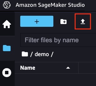
2. Start SageMaker Studio and upload the flow file to your SageMaker Studio by clicking on the upload icon highlighted in red.

Adjust transform: filter to last N-periods

In the Data Wrangler flow, you will see a transform labeled filter to last N-periods. Double-click the transform to edit it.

As delivered, this transform will compare the timestamp in the input forecast file against "today" and remove any observations prior to 36 months ago. You can wholly remove this step, or edit the time-period according to your use case. If you filter the data to very recent periods only, then quantile selection will be more sensitive to recent periods. Allowing a wider range takes a more holistic view, including viewing prior season. Apply discretion here to make the best decision for your specific case.

# this step can be used to filter backtest data to only a recent period when desired
# this allows the quantile selection to be more responsive
# CAUTION: this is defaulting to 36 months ago; change this setting accordingly

from pyspark.sql.functions import current_date, substring
from pyspark.sql import functions as F

# set working storage column
months_to_add = -36  #note negative value -N months ago
df = df.withColumn("timestamp", substring("timestamp",1,10))
df = df.withColumn("filter_date",  F.add_months("current_date", months_to_add))

# apply filter
df = df[df['timestamp']>=df['filter_date']]

# drop working storage column
df = df.drop('filter_date')

Once you have made any coding adjustments, click Preview. If the Preview is OK and shows you what you expect, click Update to add the transform in the data flow.

Adjust transform: compute-quantile-financial

As with the prior transform, you may decide to edit the quantile computation logic. This is located in a transform titled compute-quantile-financial. Here, we see an example of a dataset that shows backtest forecasted values, financial profit and loss measures, and the winner quantile (including customer override), among quantiles tested.

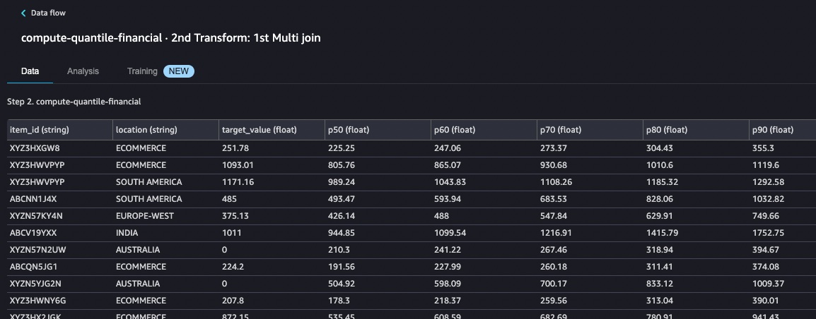
As delivered, this transform makes use of a standard set of columns in the customer provided input file. The transform also uses five quantiles, p50 through p90 in increments of 10.

At this point, you can edit the code inside Data Wrangler according to your own needs or proceed with the example use-case as delivered.

from pyspark.sql.functions import greatest, least, coalesce, round
from pyspark.sql import functions as F

quantile_list=['p50','p60','p70','p80','p90']

# compute cost of overstock (co) and cost of understock (cu)
df = df.withColumn('unit_co', (df['item_cost_of_goods'] + df['item_holding_cost']) - df['item_salvage_cost'])
df = df.withColumn('unit_cu', (df['item_value'] - df['item_cost_of_goods']))


# for each quantile compute loss function
for c in quantile_list:

  # replace negative values with zero, then round
  df.withColumn(c, F.when(df[c] < 0, 0))
  df = df.withColumn(c,round(c,2))
 
 
  # compute quantile metrics
  df = df.withColumn('co',(greatest(df[c], df.target_value) - df.target_value) * df.unit_co)
  df = df.withColumn('revenue', least(df[c], df.target_value) * df.unit_cu)
  df = df.withColumn(c+'_net', round(df.revenue + df.co,2) ) 

# initialize with fixed-quantile override
df = df.withColumn("quantile",df.fixed_quantile)

# determine greatest net revenue per quantile
df = df.withColumn("optimized_net", greatest(df.p50_net, df.p60_net, df.p70_net, df.p80_net, df.p90_net) )

# set winning quantile
for c in quantile_list:
  str = c+'_net'
  df = df.withColumn("quantile", coalesce(df.quantile, F.when( df[str] == df.optimized_net,c)))


#round target value
df = df.withColumn("target_value",round("target_value",2))

# remove undesired columns
drop_cols = ("unit_co","unit_cu","cu","co", "optimized_net", "revenue")
df = df.drop(*drop_cols) 

Once you have made any coding adjustments, click Preview. If the Preview is OK and shows you what you expect, click Update to add the transform in the data flow.

Create your S3 output destinations

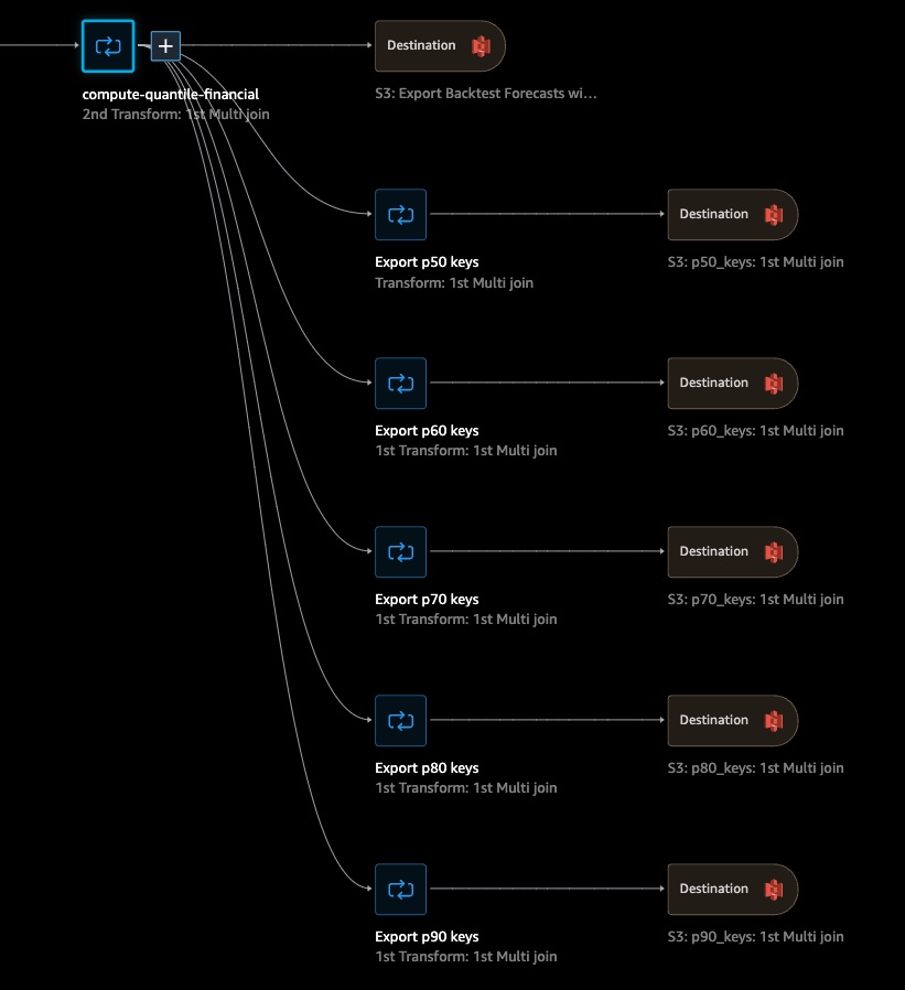
As delivered, the solution has no S3 destinations. As shown in the picture below, you can setup S3 locations where the results of each transform can be saved for subsequent use in your data pipeline. In this section, the goal is to add S3 destinations, which ultimately, will write data to your own S3 bucket. In this example, the goal is to add multiple destinations to your sample Data Wrangler workflow as follows.

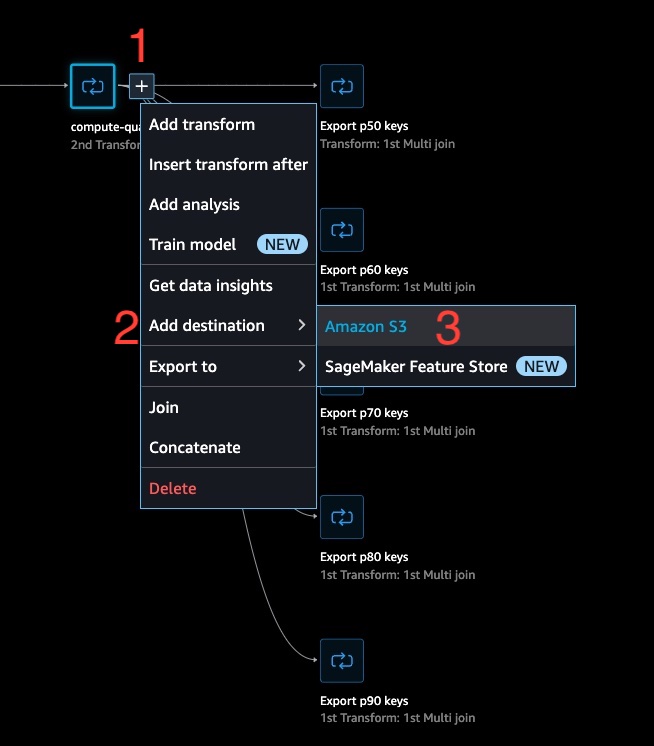
1. Click the (+) on the transform titled compute-quantile-financials, then click Add Destination and choose Amazon S3.

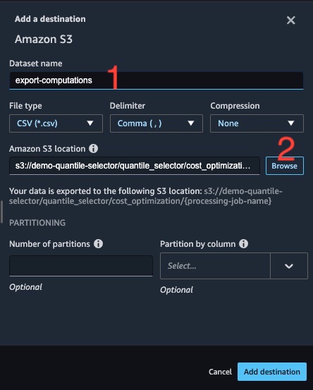
2. At the next screen, provide a meaningful dataset name then use the browse button to locate where you want the output file written in your AWS environment. In this step, be sure to select your own S3 bucket else you might have a failure.

3. The CSV output files per quantile are also designed to be written to S3 as a list of item_id and region values. You may not need the quantile based output files and can delete these, if appropriate. The purpose of these distinct files is to use them to drive Amazon Forecast such that it produces future forecasts, at specific quantiles, for named items as a cost efficiency measure. Please read our blog for more information at Choose specific timeseries to forecast with Amazon Forecast.

Scheduling the transformation

Next, this process demonstrates how to execute the transformation. Ideally, in future periods, as long as your input files are updated, you are able to get automatic output files to be used as part of your workflow or analyses.

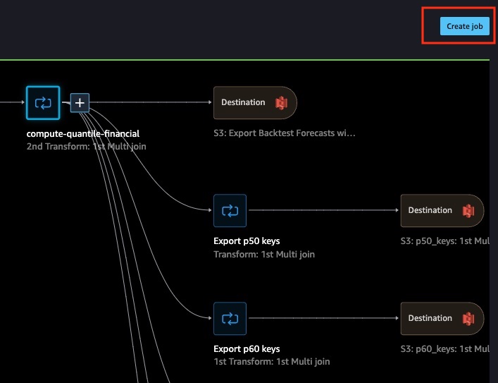
1. Locate the blue Create Job button on the top-right of the screen as shown.

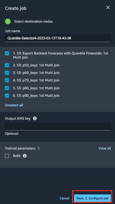
2. You may provide a unique job name here, or unselect destinations if applicable.

3. Click click the blue box at the bottom to proceed forward.

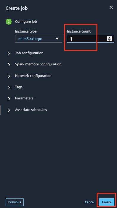
4. At the Create Job step, change instance count to 1, until you find your task is too big to fit on single nodes.

5. Click Create to proceed.

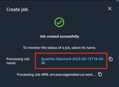
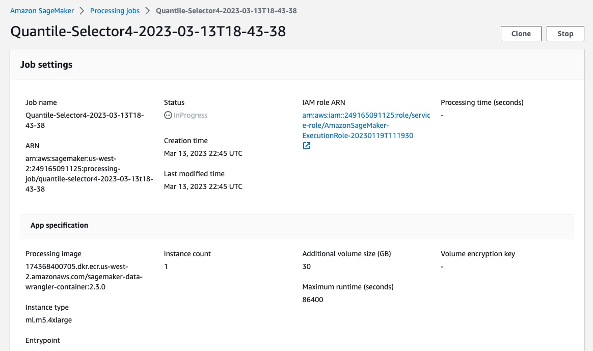
6. This provides you with confirmation the processing job has started. Click on the URL here to monitor the job.

7. Once the processing job completes, the status will become "Complete". You can view the output files created at the S3 locations described in the transformation job.

Conclusion

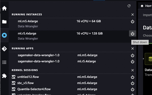
Once you have completed the process, you should take care to stop the SageMaker Data Wranger instance from SageMaker Studio. In the screenshot provided, click on the power button icon beside the list of SageMaker Data Wrangler instances. Ongoing you do not need to use the user interface, unless you want to alter a flow. If you want to transform data on a recurring basis, you may reuse the flow file, which now resides on S3.

Please let your AWS account team or your AWS solution architect know if you have any questions about this end-to-end process.