iphones_R00 sc.parallelize ([
  (XS, 2018, 5.65, 2.79, 6.24),
  (XR", 2018, 5.94, 2.98, 6.84),
  (X10, 2017, 5.65, 2.79, 6.13),
  (8PLUS, 2017, 6.23, 3.07, 7.12)
])

names ["Model", "Year", "Height", "Width", "Weight"]

iphones_df = spark.createDataFrame (iphones_RDD, schema=names)
type(iphones_df)
pyspark. sql.dataframe . DataFrame
df_csv spark. read.csv("people. csv", header=True , inferSchema=True)
df_json spark.read.json("people . json", header=True, inferSchema=True)
df txt= spark. read. txt("people. txt", header=True, inferSchema= True)- Path to the file and two optional parameters
- Two optional parameters
header=True, inferSchema=True
Instructions
- Create an RDD from the sample_list.
- Create a PySpark DataFrame using the above RDD and schema.
- Confirm the output as PySpark DataFrame.
# Create a list of tuples
sample_list = [('Mona',20), ('Jennifer',34), ('John',20), ('Jim',26)]

# Create an RDD from the list
rdd = sc.parallelize(sample_list)

# Create a PySpark DataFrame
names_df = spark.createDataFrame(rdd, schema=['Name', 'Age'])

# Check the type of names_df
print("The type of names_df is", type(names_df))

# The type of names_df is <class 'pyspark.sql.dataframe.DataFrame'>Instructions
- Create a DataFrame from file_path variable which is the path to the people.csv file.
- Confirm the output as PySpark DataFrame.
# Create an DataFrame from file_path # people.csv
people_df = spark.read.csv(file_path, header=True, inferSchema=True)

# Check the type of people_df
print("The type of people_df is", type(people_df))

# The type of people_df is <class 'pyspark.sql.dataframe.DataFrame'>Instructions
- Print the first 10 observations in the people_df DataFrame.
- Count the number of rows in the people_df DataFrame.
- How many columns does people_df DataFrame have and what are their names?
# Print the first 10 observations
people_df.show(10)

# Count the number of rows
print("There are {} rows in the people_df DataFrame.".format(people_df.count()))

# Count the number of columns and their names
print("There are {} columns in the people_df DataFrame and their names are {}".format(len(people_df.columns), people_df.columns))

''' result :

There are 100000 rows in the people_df DataFrame.
There are 5 columns in the people_df DataFrame and their names are ['_c0', 'person_id', 'name', 'sex', 'date of birth']
'''- Select 'name', 'sex' and 'date of birth' columns from people_df and create people_df_sub DataFrame.
- Print the first 10 observations in the people_df DataFrame.
- Remove duplicate entries from people_df_sub DataFrame and create people_df_sub_nodup DataFrame.
- How many rows are there before and after duplicates are removed?
# Select name, sex and date of birth columns
people_df_sub = people_df.select('name', 'sex', 'date of birth')

# Print the first 10 observations from people_df_sub
people_df_sub.show(10)

# Remove duplicate entries from people_df_sub
people_df_sub_nodup = people_df_sub.dropDuplicates()

# Count the number of rows
print("There were {} rows before removing duplicates, and {} rows after removing duplicates".format(people_df_sub.count(), people_df_sub_nodup.count()))

# There were 100000 rows before removing duplicates, and 99998 rows after removing duplicates- Filter the people_df DataFrame to select all rows where sex is female into people_df_female DataFrame.
- Filter the people_df DataFrame to select all rows where sex is male into people_df_male DataFrame.
- Count the number of rows in people_df_female and people_df_male DataFrames.
# Filter people_df to select females
people_df_female = people_df.filter(people_df.sex == "female")

# Filter people_df to select males
people_df_male = people_df.filter(people_df.sex == "male")

# Count the number of rows
print("There are {} rows in the people_df_female DataFrame and {} rows in the people_df_male DataFrame".format(people_df_female.count(), people_df_male.count()))

# There are 49014 rows in the people_df_female DataFrame and 49066 rows in the people_df_male DataFrame- Create a temporary table people that's a pointer to the people_df DataFrame.
- Construct a query to select the names of the people from the temporary table people.
- Assign the result of Spark's query to a new DataFrame - people_df_names.
- Print the top 10 names of the people from people_df_names DataFrame.
# Create a temporary table "people"
people_df.createOrReplaceTempView("people")

# Construct a query to select the names of the people from the temporary table "people"
query = '''SELECT name FROM people'''

# Assign the result of Spark's query to people_df_names
people_df_names = spark.sql(query)

# Print the top 10 names of the people
people_df_names.show(10)

'''
+----------------+
|            name|
+----------------+
|  Penelope Lewis|
|   David Anthony|
|       Ida Shipp|
|    Joanna Moore|
|  Lisandra Ortiz|
|   David Simmons|
|   Edward Hudson|
|    Albert Jones|
|Leonard Cavender|
|  Everett Vadala|
+----------------+
'''- Filter the people table to select all rows where sex is female into people_female_df DataFrame.
- Filter the people table to select all rows where sex is male into people_male_df DataFrame.
- Count the number of rows in both people_female and people_male DataFrames.
# Filter the people table to select female sex
people_female_df = spark.sql('SELECT * FROM people WHERE sex=="female"')

# Filter the people table DataFrame to select male sex
people_male_df = spark.sql('SELECT * FROM people WHERE sex=="male"')

# Count the number of rows in both DataFrames
print("There are {} rows in the people_female_df and {} rows in the people_male_df DataFrames".format(people_female_df.count(), people_male_df.count()))

# There are 49014 rows in the people_female_df and 49066 rows in the people_male_df DataFrames- Print the names of the columns in names_df DataFrame.
- Convert names_df DataFrame to df_pandas Pandas DataFrame.
- Use matplotlib's plot() method to create a horizontal bar plot with 'Name' on x-axis and 'Age' on y-axis.
# Check the column names of names_df
print("The column names of names_df are", names_df.columns)

# Convert to Pandas DataFrame
df_pandas = names_df.toPandas()

# Create a horizontal bar plot
df_pandas.plot(kind='barh', x='Name', y='Age', colormap='winter_r')
plt.show()
- Create a PySpark DataFrame from file_path (which is the path to the Fifa2018_dataset.csv file).
- Print the schema of the DataFrame.
- Print the first 10 observations.
- How many rows are in there in the DataFrame?
# Load the Dataframe
fifa_df = spark.read.csv(file_path, header=True, inferSchema=True)

# Check the schema of columns
fifa_df.printSchema()

# Show the first 10 observations
fifa_df.show(10)

# Print the total number of rows
print("There are {} rows in the fifa_df DataFrame".format(fifa_df.count()))

''' showing schema :
 |-- _c0: integer (nullable = true)
 |-- Name: string (nullable = true)
 |-- Age: integer (nullable = true)
 |-- Photo: string (nullable = true)
 |-- Nationality: string (nullable = true)......
# showing 10 rows
# There are 17981 rows in the fifa_df DataFrame
'''- Create temporary table fifa_df from fifa_df_table DataFrame.
- Construct a "query" to extract the "Age" column from Germany players.
- Apply the SQL "query" to the temporary view table and create a new DataFrame.
- Computes basic statistics of the created DataFrame.
# Create a temporary view of fifa_df
fifa_df.createOrReplaceTempView('fifa_df_table')

# Construct the "query"
query = '''SELECT * FROM fifa_df_table WHERE Nationality == "Germany"'''

# Apply the SQL "query"
fifa_df_germany_age = spark.sql(query)

# Generate basic statistics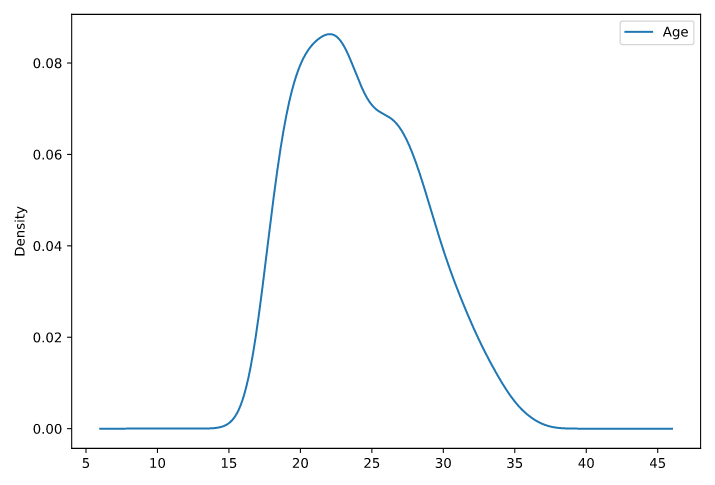
fifa_df_germany_age.describe().show()- Convert fifa_df_germany_age to fifa_df_germany_age_pandas Pandas DataFrame.
- Generate a density plot of the 'Age' column from the fifa_df_germany_age_pandas Pandas DataFrame.
# Convert fifa_df to fifa_df_germany_age_pandas DataFrame
fifa_df_germany_age_pandas = fifa_df_germany_age.toPandas()

# Plot the 'Age' density of Germany Players
fifa_df_germany_age_pandas.plot(kind='density')
plt.show()