clt: an R package for demonstrating the central limit theorem

clt runs Monte Carlo simulations for a given inverse cdf and outputs z-scores for each N and simulation to a data frame. You can install it using devtools:

devtools::install_github("dfsnow/clt")

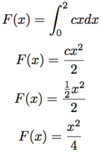
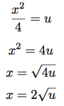
For example, here's a basic linear cdf and inverse cdf:

clt()

Given the inverse cdf above, you can run Monte Carlo simulations for various sample sizes of N using clt(). N is a vector of integers representing the number of draws from a distribution, B is the number of times one simulates each draw, and mu is the known mean of the pdf. Note that the inverse cdf argument is a string. The output is a dataframe with the dimensions length(N) x B.

clt(N = c(15,30,60,120,240,500), invcdf = "2*sqrt(runif(n))", B = 1000, mu = (4/3))

clt_eval()

The clt_eval() function can be used to evaluate the output of the Monte Carlo simulations. It calculates the percentage of z-scores beyond the specified critical value. As N increases all distributions should become approximately normal. Thus, with critical values of 1.96, all distributions sampled at large N should have roughly 5% of their data beyond the critical threshold. Here's an example of clt_eval in action:

clt(N = 2:50, invcdf = "runif(n, -1, 1)", B = 10000) %>% clt_eval()

This will draw N times from a uniform distrubtion, from N = 2 to N = 50, . This will very quickly approximate a normal distribution.

clt_anim()

Note: ImageMagick must be installed for this function to work.

The clt_anim() function animates the results of clt() and outputs a gif file. It uses ggplot2 to plot the z-scores for each N value in a density histogram, and treats each N as a frame. ImageMagick and the magick package are used to compile each frame into a gif. You can install ImageMagick using:

brew install imagemagick

You can also use the pipe operator to pipe the results of clt() directly to clt_anim(). See examples:

Uniform Distribution

clt(N = c(2,4,8,16,32,64,128,256,512,1024,2048,4096,8192,16384),
  invcdf = "runif(n, -1, 1)", B = 10000) %>%
clt_anim(compile = TRUE, fps = 2, xlim = c(-4, 4))

Binomial Distribution

clt(N = c(2,4,8,16,32,64,128,256,512,1024,2048,4096,8192,16384),
  invcdf = "ifelse(runif(n) < .75, 1, 0)", B = 10000, mu = .75) %>%
clt_anim(compile = TRUE, fps = 2)

Log Normal Distribution

clt(N = c(2,4,8,16,32,64,128,256,512,1024,2048,4096,8192,16384),
  invcdf = "exp(1 + qnorm(runif(n)))", B = 10000, mu = 4.48) %>%
clt_anim(compile = TRUE, fps = 2, xlim = c(-8, 4))

Exponential Distribution

clt(N = c(2,4,8,16,32,64,128,256,512,1024,2048,4096,8192,16384),
  invcdf = "qexp(runif(n), .10)", B = 10000, mu = 10) %>%
clt_anim(compile = TRUE, fps = 2, xlim = c(-8, 4))