-
Notifications
You must be signed in to change notification settings - Fork 0
/
slides.qmd
708 lines (496 loc) · 17.9 KB
/
slides.qmd
1
2
3
4
5
6
7
8
9
10
11
12
13
14
15
16
17
18
19
20
21
22
23
24
25
26
27
28
29
30
31
32
33
34
35
36
37
38
39
40
41
42
43
44
45
46
47
48
49
50
51
52
53
54
55
56
57
58
59
60
61
62
63
64
65
66
67
68
69
70
71
72
73
74
75
76
77
78
79
80
81
82
83
84
85
86
87
88
89
90
91
92
93
94
95
96
97
98
99
100
101
102
103
104
105
106
107
108
109
110
111
112
113
114
115
116
117
118
119
120
121
122
123
124
125
126
127
128
129
130
131
132
133
134
135
136
137
138
139
140
141
142
143
144
145
146
147
148
149
150
151
152
153
154
155
156
157
158
159
160
161
162
163
164
165
166
167
168
169
170
171
172
173
174
175
176
177
178
179
180
181
182
183
184
185
186
187
188
189
190
191
192
193
194
195
196
197
198
199
200
201
202
203
204
205
206
207
208
209
210
211
212
213
214
215
216
217
218
219
220
221
222
223
224
225
226
227
228
229
230
231
232
233
234
235
236
237
238
239
240
241
242
243
244
245
246
247
248
249
250
251
252
253
254
255
256
257
258
259
260
261
262
263
264
265
266
267
268
269
270
271
272
273
274
275
276
277
278
279
280
281
282
283
284
285
286
287
288
289
290
291
292
293
294
295
296
297
298
299
300
301
302
303
304
305
306
307
308
309
310
311
312
313
314
315
316
317
318
319
320
321
322
323
324
325
326
327
328
329
330
331
332
333
334
335
336
337
338
339
340
341
342
343
344
345
346
347
348
349
350
351
352
353
354
355
356
357
358
359
360
361
362
363
364
365
366
367
368
369
370
371
372
373
374
375
376
377
378
379
380
381
382
383
384
385
386
387
388
389
390
391
392
393
394
395
396
397
398
399
400
401
402
403
404
405
406
407
408
409
410
411
412
413
414
415
416
417
418
419
420
421
422
423
424
425
426
427
428
429
430
431
432
433
434
435
436
437
438
439
440
441
442
443
444
445
446
447
448
449
450
451
452
453
454
455
456
457
458
459
460
461
462
463
464
465
466
467
468
469
470
471
472
473
474
475
476
477
478
479
480
481
482
483
484
485
486
487
488
489
490
491
492
493
494
495
496
497
498
499
500
501
502
503
504
505
506
507
508
509
510
511
512
513
514
515
516
517
518
519
520
521
522
523
524
525
526
527
528
529
530
531
532
533
534
535
536
537
538
539
540
541
542
543
544
545
546
547
548
549
550
551
552
553
554
555
556
557
558
559
560
561
562
563
564
565
566
567
568
569
570
571
572
573
574
575
576
577
578
579
580
581
582
583
584
585
586
587
588
589
590
591
592
593
594
595
596
597
598
599
600
601
602
603
604
605
606
607
608
609
610
611
612
613
614
615
616
617
618
619
620
621
622
623
624
625
626
627
628
629
630
631
632
633
634
635
636
637
638
639
640
641
642
643
644
645
646
647
648
649
650
651
652
653
654
655
656
657
658
659
660
661
662
663
664
665
666
667
668
669
670
671
672
673
674
675
676
677
678
679
680
681
682
683
684
685
686
687
688
689
690
691
692
693
694
695
696
697
698
699
700
701
702
703
704
705
706
707
708
---
title: "Introduction to reproducible data analysis with R and Quarto"
title-slide-attributes:
data-background-color: "#a13c65"
data-background-image: "images/LMU_Logo.png"
data-background-size: 15%
data-background-position: 50% 83%
subtitle: "KLI Seminar 2023"
author:
- name: Anne-Kathrin Kleine
format:
revealjs:
slide-number: true
width: 1500
height: 1000
chalkboard:
buttons: false
preview-links: false
footer: <https://quarto.org>
theme: [simple, custom.scss]
logo: "images/LMU_Logo.png"
scrollable: false
center: true
incremental: false
link-external-newwindow: true
resources:
- demo.pdf
---
```{r include=FALSE}
library(fontawesome)
library(tidyverse)
library(quarto)
library(gt)
library(gtExtras)
```
# Schedule {background-color="#a13c65"}
## DAY 1
::: fragment
### 9.00-9.30: Introduction
- Welcome and overview
- Reproducibility and open science
:::
::: fragment
### 9.40-10.30: Getting Started with R and Quarto
- Best practices for organizing your code and materials
- File and folder structure
:::
------------------------------------------------------------------------
### 11.00-12.00: Creating data analysis projects in R and quarto
- Basics of R programming
- Creating a data analysis project
- Integrating code, text, and output within a Quarto document
::: fragment
### 12.15-13.00: Working with data
- Working with data in R: importing, manipulating, and exporting data
- Data visualization and data analysis
:::
## DAY 2
::: fragment
### 09.00-10.00: Publishing Reproducible Data Analysis Scripts
- Sharing your scripts and data
- Publishing through GitHub, RPubs; integration with osf
:::
::: fragment
### 10.15-11.00: Hands-on Practice PART I
- Guided exercise: Data analysis project using R and Quarto
- Independent practice: Working on your data analysis project with support from workshop facilitator
:::
------------------------------------------------------------------------
### 11.30-12.15: Hands-on Practice PART II
::: fragment
### 12.00-13.00: Closing Remarks and Resources
- Recap of the workshop
- Additional resources for learning R, Quarto, reproducibility best practices, version control and collaboration
- Q&A session
:::
## Workshop Requirements
- Are you on the [latest version of RStudio](https://posit.co/download/rstudio-desktop/#download)?
. . .
- Open RStudio
------------------------------------------------------------------------
## Install relevant packages
```{r}
#| echo: fenced
#| eval: false
pkg_list <- c("tidyverse", "haven", "flextable", "broom", "report", "effectsize", "rempsyc")
install.packages(pkg_list)
```
# Reproducibility and open science {background-color="#a13c65"}
------------------------------------------------------------------------
## Reproducibility and replicability
::: callout-tip
## Reproducibility
**Reproducibility** means that research data and code are made available so that others are able to reach the same results as are claimed in scientific outputs. Closely related is the concept of **replicability**, the act of repeating a scientific methodology to reach similar conclusions. These concepts are core elements of empirical research.
::: fragment
Reproducibility emphasizes re-using original data and methods for verification, while replicability focuses on achieving consistent results with repeats of the experiment under similar conditions but using new data.
:::
:::
::: {style="font-size: 50%;"}
From [The Open Science Training Handbook](https://open-science-training-handbook.github.io/Open-Science-Training-Handbook_EN/02OpenScienceBasics/04ReproducibleResearchAndDataAnalysis.html)
:::
------------------------------------------------------------------------
## Open Science for ensuring reproducibility and replicability

::: {style="font-size: 50%;"}
Source: [The six core principles of Open Science](https://www.researchgate.net/figure/The-six-core-principles-of-Open-Science-which-guide-the-Open-Traits-Network_fig1_332352194)
:::
------------------------------------------------------------------------
## The benefits of Open Science for behavioral researchers

::: {style="font-size: 50%;"}
Source: [The benefits of Open Science](https://phoebekoundouri.org/what-is-open-science/)
:::
## The role of R and Quarto (RMarkdown) for Open Science
::: fragment
### R and Quarto are open-source
- ensuring accessibility, collaboration, customizability, longevity
:::
::: fragment
### Producing shareable and collaborative high-quality documents that integrate text and R code for analysis and visualization within one document
:::
::: fragment
- minimize "false" results in output documents because nothing needs to be copy-pasted
- "coding" of research papers (easy integration of later modifications)
:::
# Change Your Mental Model {background-color="#a13c65"}
##
::: columns
::: {.column width="50%"}
Source
{width="700px" fig-alt="A blank Word document"}
:::
::: {.column width="50%"}
Output
{width="700px" fig-alt="A blank Word document"}
:::
:::
##
::: columns
::: {.column width="50%"}
Source
````
---
title: "ggplot2 demo"
author: "Norah Jones"
date: "5/22/2021"
format:
html:
fig-width: 8
fig-height: 4
code-fold: true
---
## Air Quality
@fig-airquality further explores the impact of temperature
on ozone level.
```{{r}}
#| label: fig-airquality
#| fig-cap: Temperature and ozone level.
#| warning: false
library(ggplot2)
ggplot(airquality, aes(Temp, Ozone)) +
geom_point() +
geom_smooth(method = "loess"
)
```
````
:::
::: {.column width="50%"}
Output 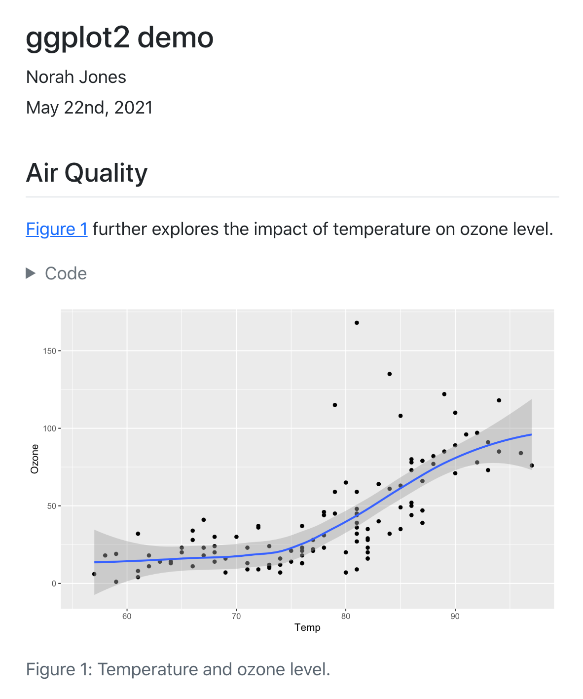
:::
:::
# Getting Started with R {background-color="#a13c65"}
## [Getting Started with R](https://rafalab.dfci.harvard.edu/dsbook/getting-started.html)

# Creating a data analysis project {background-color="#a13c65"}
## Create a folder for your R project

------------------------------------------------------------------------
## Create a Quarto document (report.qmd)

------------------------------------------------------------------------
## Create an R project

------------------------------------------------------------------------
## R projects
When a project is opened within RStudio the following actions are taken:
. . .
- A new R session is started
. . .
- The .Rprofile, .RData file, and .Rhistory files in the project's main directory are loaded
. . .
- **The current working directory is set to the project directory**
. . .
- Previously edited source documents are restored into editor tabs
. . .
- Other RStudio settings (e.g. active tabs, splitter positions, etc.) are restored to where they were the last time the project was closed
# Working with Quarto {background-color="#a13c65"}
## How does Quarto work?
{fig-alt="A diagram of how a RMD is turned into output formats via knitr and pandoc"}
------------------------------------------------------------------------
## So what is Quarto?
> Quarto is a command line interface (CLI) that renders plain text formats (`.qmd`, `.rmd`, `.md`) into static PDF/Word/HTML reports, books, websites, presentations and more
## One install, "Batteries included"
- Quarto is bundled and comes pre-installed with RStudio [v2022.07.1](https://www.rstudio.com/products/rstudio/download/#download) and beyond!
- [more infos](https://quarto.org/docs/computations/r.html#installation)
## Rendering
1. Render button
. . .
{fig-alt="A screenshot of the render button in RStudio" width="1000px"}
## Rendering
2. System shell via `quarto render`
::: {style="font-size: 60px;"}
``` {.bash filename="terminal"}
quarto render document.qmd # defaults to html
quarto render document.qmd --to pdf
quarto render document.qmd --to docx
```
:::
------------------------------------------------------------------------
### Quick excourse: *Power Shell* and *Terminal* {background-color="#DADEFD"}
::: columns
::: {.column width="50%"}
[Windows Power Shell](https://learn.microsoft.com/en-us/powershell/scripting/discover-powershell?view=powershell-7.2)
- Click Start, type PowerShell, right-click Windows PowerShell, and then click Run as administrator
{width="600px"}
[Image source: Wikipedia](https://upload.wikimedia.org/wikipedia/de/f/f6/Windowspowershell_unter_Windows_8.png)
:::
::: {.column width="50%"}
[Mac Terminal](https://support.apple.com/en-gb/guide/terminal/apd5265185d-f365-44cb-8b09-71a064a42125/mac)
- Click the Launchpad icon in the Dock, type Terminal in the search field, then click Terminal
{width="700px"}
[Image source: Wikipedia](https://en.wikipedia.org/wiki/Terminal_(macOS)#/media/File:Appleterminal2.png)
:::
:::
## Rendering
3. R console via `quarto` R package
::: {style="font-size: 60px;"}
```{r}
#| eval: false
#| echo: fenced
library(quarto)
quarto_render("document.qmd") # defaults to html
quarto_render("document.qmd", output_format = "pdf")
```
:::
# Working with a `.qmd` {background-color="#a13c65"}
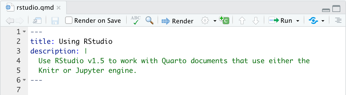
## A `.qmd` is a plain text file
. . .
- Metadata (YAML)
::: {style="font-size: 60px;"}
``` yaml
format: html
engine: knitr
```
:::
. . .
- Code
::: {style="font-size: 60px;"}
```{{r}}
library(dplyr)
mtcars |>
group_by(cyl) |>
summarize(mean = mean(mpg))
```
:::
. . .
- Text
::: {style="font-size: 60px;"}
``` markdown
# Heading 1
This is a sentence with some **bold text**, *italic text* and an
{fig-alt="Alt text for this image"}.
```
:::
## Metadata: YAML
The [YAML](https://yaml.org/) metadata or header is:
> influences the final document in different ways. It is placed at the very beginning of the document and is read by each of Pandoc, Quarto and `knitr`. Along the way, the information that it contains can affect the code, content, and the rendering process.
## YAML
::: {style="font-size: 70px;"}
``` yaml
title: "My Document"
format:
html:
toc: true
code_folding: 'show'
```
:::
See more formats and other YAML metadata options [here](https://quarto.org/docs/output-formats/all-formats.html)
## Why YAML?
To avoid manually typing out all the options, every time!
. . .
::: {style="font-size: 70px;"}
``` {.bash filename="terminal"}
quarto render document.qmd --to html
```
:::
<br>
. . .
::: {style="font-size: 70px;"}
``` {.bash filename="terminal"}
quarto render document.qmd --to html -M code fold:true
```
:::
<br>
. . .
::: {style="font-size: 70px;"}
``` {.bash filename="terminal"}
quarto render document.qmd --to html -M code-fold:true -P alpha:0.2 -P ratio:0.3
```
:::
## Quarto workflow
Executing the Quarto Render button in RStudio will call Quarto render in a background job - this will prevent Quarto rendering from cluttering up the R console, and gives you and easy way to stop.

## Markdown
> Quarto uses markdown as its underlying document syntax. Markdown is a plain text format that is designed to be easy to write, and, even more importantly, easy to read
## Text Formatting
+-----------------------------------+-------------------------------+
| Markdown Syntax | Output |
+===================================+===============================+
| ``` | *italics* and **bold** |
| *italics* and **bold** | |
| ``` | |
+-----------------------------------+-------------------------------+
| ``` | superscript^2^ / subscript~2~ |
| superscript^2^ / subscript~2~ | |
| ``` | |
+-----------------------------------+-------------------------------+
| ``` | ~~strikethrough~~ |
| ~~strikethrough~~ | |
| ``` | |
+-----------------------------------+-------------------------------+
| ``` | `verbatim code` |
| `verbatim code` | |
| ``` | |
+-----------------------------------+-------------------------------+
## Headings
+-------------------+-----------------+
| Markdown Syntax | Output |
+===================+=================+
| ``` | # Header 1 |
| # Header 1 | |
| ``` | |
+-------------------+-----------------+
| ``` | ## Header 2 |
| ## Header 2 | |
| ``` | |
+-------------------+-----------------+
| ``` | ### Header 3 |
| ### Header 3 | |
| ``` | |
+-------------------+-----------------+
| ``` | #### Header 4 |
| #### Header 4 | |
| ``` | |
+-------------------+-----------------+
## Code
```{r}
#| echo: fenced
#| output-location: column
#| fig-cap: Temperature and ozone level.
#| warning: false
library(ggplot2)
ggplot(airquality, aes(Temp, Ozone)) +
geom_point() +
geom_smooth(method = "loess")
```
# Data importing, manipulating, and exporting {background-color="#a13c65"}
## Get data
- Download [the example dataset](https://github.com/AnneOkk/attitudes_study/tree/main/Data)
- Store data file in "data/raw" folder
## Reading data in
```{r}
#| echo: fenced
## Read in data
library(readxl)
library(tidyverse)
data <- read_excel("Exercise/data/raw/data.xlsx", col_names = T) # if you created an R project you can use the direct path "data/raw/data.xlsx"
```
## Manipulating data
```{r}
#| echo: fenced
# Name correction
names(data) <- gsub("d2priv", "dapriv2", names(data))
# Own function
recode_5 <- function(x) {
x * (-1)+6
}
# Use of mutate_at to apply function
data_proc <- data %>%
mutate_at(vars(matches("gattAI1_3|gattAI1_6|gattAI1_8|gattAI1_9|gattAI1_10|gattAI2_5|gattAI2_9|gattAI2_10")), recode_5)
```
## Exporting data
```{r}
#| echo: fenced
library(haven)
write_sav(data_proc, "Exercise/data/processed/data_proc.sav") # if you created an R project you can use the direct path "data/processed/data_proc.sav"
```
# The R folder {background-color="#a13c65"}
## Storing and sourcing custom functions from the R folder
- You may store your custom functions in a separate file (e.g., "R/custom-functions.R") that you may source in your report document ("report.qmd")
**In R/custom-functions.R**:
```{r}
#| echo: fenced
# Own function
recode_5 <- function(x) {
x * (-1)+6
}
```
**Reading in your custom functions**:
```{r}
#| echo: fenced
source("Exercise/R/custom-functions.R")
```
# Tables and visualisations {background-color="#a13c65"}
## Reading in data
```{r}
#| echo: fenced
data <- haven::read_sav("Exercise/data/processed/data_proc.sav")
```
## Creating a correlation table
### Creating composites
```{r}
#| echo: fenced
data <- data[ , purrr::map_lgl(data, is.numeric)] %>% # select numeric variables
select(matches("gattAI1|soctechblind|trust1|anxty1|SocInf1|Age")) # select relevant variables
comp_split <- data %>% sjlabelled::remove_all_labels(.) %>%
split.default(sub("_.*", "", names(data))) # creating a list of dataframes, where each dataframe consists of the columns from the original data that shared the same prefix (all characters before the underscore)
comp <- purrr::map(comp_split, ~ rowMeans(.x, na.rm=T)) #calculating the row-wise mean of each data frame in the list `comp_split`, with the output being a new list (`comp`) where each element is a numeric vector of row means from each corresponding data frame in `comp_split`
comp_df <- do.call("cbind", comp) %>% as.data.frame(.) # binding all the elements in the list `comp` into a single data frame, `comp_df`
```
## Creating the correlation table
```{r}
#| echo: fenced
cor_tab <- corstars(comp_df, removeTriangle = "upper")
cor_tab
```
## Creating correlation plot
```{r}
#| echo: fenced
cor_matrix <- cor(comp_df[1:6])
corrplot::corrplot(cor_matrix, method="color", type="upper", order="hclust",
addCoef.col = "black", # Add correlation coefficient on the plot
tl.col="black", # Text label color
tl.srt=90, # Text label rotation
title="Correlation matrix", mar=c(0,0,1,0))
```
## Scatterplot
```{r}
#| echo: fenced
scatter <- ggplot(comp_df, aes(x=SocInf1, y=trust1, color=Age)) +
geom_point() +
labs(x="Anxiety", y="GattAI1", color="Age") +
theme_minimal() +
ggtitle("Scatterplot of social influence and trust colored by age")
scatter
```
## Saving scatterplot
```{r}
#| echo: fenced
ggsave(filename="Exercise/output/figs/scatter.png", plot=scatter)
```
# Referencing, style and the config folder {background-color="#a13c65"}
## Bibliography and csl style documents
::: {style="font-size: 60px;"}
``` yaml
___
bibliography: "/config/refs.bib"
csl: "/config/apa.csl"
---
```
:::

## Select a csl style
[Zotero Style Repository](https://www.zotero.org/styles?q=APA)

## Store a template word document
::: {style="font-size: 60px;"}
``` yaml
format:
docx:
reference-doc: "/config/template_apa.docx"
```
:::
# Folder structure overview {background-color="#a13c65"}
## Current folder structure

## Back to "report.qmd"
. . .
### The visual editor and inserting text and citations

# Questions and outlook
## Questions?
## Outlook
- Tomorrow we will look into data analysis publication for true reproducibility
. . .
- You will get the chance to work on your own data analysis project or use the material provided