Beginner's Tutorial (short version)
In this tutorial, we will use the BEAST 2 package MultiTypeTree to perform a Bayesian phylogenetic analysis of an influenza data set using the structured coalescent model.
The data set used in this tutorial is a thinned (60 sequence) subset of the (980 sequence) data set used in the publication Vaughan et al., 2014, which in turn was assembled from publicly-available data sets provided by various authors on GenBank.
In order to proceed, ensure you have the latest version (currently 2.4) of BEAST 2 installed. To analyze the inference results you'll also need a recent versions of Tracer and an up-to-date version of Google Chrome or Mozilla Firefox.
You can easily install this package via BEAUti's package manager. To do this, follow these steps:
- Start BEAUti
- From the File menu, select Manage packages.
- Find "MultiTypeTree" in the list of packages shown, select it and then click "Install/Upgrade":
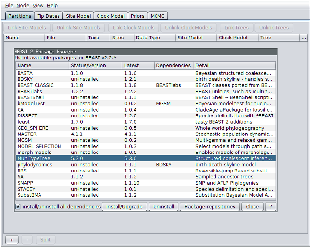
(Note the actual version of MultiTypeTree may differ from the version shown in the figure. This is normal.)
Finally, restart BEAUti. This is very important. Strange behaviour will result if you do not restart the program.
From the File menu, select Template and then choose MultiTypeTree:

Once the template is loaded, we can load in our example sequence data. In our case, this data is stored a FASTA file, the first few lines of which look like this:
> EU856841_HongKong_2005.34246575
-----------GGGATAATTCTATTAACCATGAAGACTATCATTGCTTTGAGCTACATTT
> EU856989_HongKong_2002.58356164
--CAAAAGCAGGGGATAATTCTATTAACCATGAAGACTATCATTGCTTTGAGCTACATTT...
> CY039495_HongKong_2004.5890411
------------------TTCTATTAACCATGAAGACTATCATTGCTTTGAGCTACATTC...
> EU856853_HongKong_2001.17808219
---------------------TATTAACCATGAAGACTATCATTGCTTTGAGCTACATTC...
> CY010084_NewZealand_2005.62739726
---------------------TATTAACCATGAAGACTATCATTGCTTTGAGCTACATTC...
> CY007387_NewZealand_2004.63287671
---------------------TATTAACCATGAAGACTATCATTGCTTTGAGCTACATTC...
> CY012432_NewZealand_2000.81643836
---------------------------CCATGAAGACTATCATTGCTTTGAGCTACATTT...
The lines beginning with ">" are labels for the sequences immediately following. In general, these labels have no special format, but in this file each label is a underscore-delimited triple. The first element of each triple is the GenBank accession number of the sequence, the second is the geographical region from which it was sampled, and the third is the time at which it was sampled measured in calendar years or fractions thereof. (The ellipses are not in the file, but are used here to indicate that sequence has been truncated.)
In this tutorial we will be using the influenza sequence data which is
distributed with MultiTypeTree. To make this easy to find, open the File
menu and select Set working dir. Then, from the submenu that appears, select
MultiTypeTree.

(This step is not required when loading your own data.)
To load the file, open the File menu and select Add alignment. This
will open a file selection dialog box. The example influenza sequence data
file is named h3n2_2deme.fna. Assuming you have followed the previous step to set
the working directory, this can be found in the examples/ directory shown
when the file selection dialog box loads.
Once this file is loaded, your BEAUti screen should look something like the following:

Once the data is loaded, the next step is to specify the times at which the sequences were sampled:
- Select the "Tip Dates" panel.
- Check the "use tip dates" checkbox.
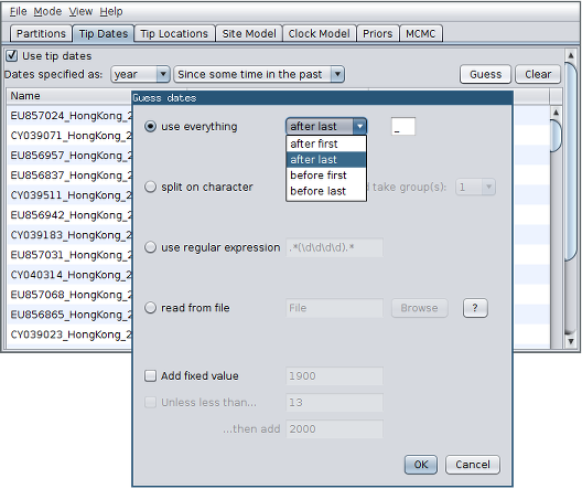
- Click the "Auto-configure" button at the top-right of the panel. This opens a dialog that allows sample times to be loaded from a file or inferred (guessed) from the sequence labels.
- Because the times are included as the last element of the underscore-delimited triple in the header, choose the "use everything" radio button and select "after last" from the drop-down menu. (Note that the underscore character is already chosen as the delimiter.)
After clicking "OK" you should find that the tip date table is populated with times that match those in the sequence headers, and that the last column of the table contains "heights" (times before most recent sample) calculated from the times:

Now we've specified the sampling times, we move on to specifying the sampling locations. To do this, we follow a very similar set of steps to those we used to set the sample times:
- Select the "Tip Locations" panel. You'll find that the locations are already populated with default values.
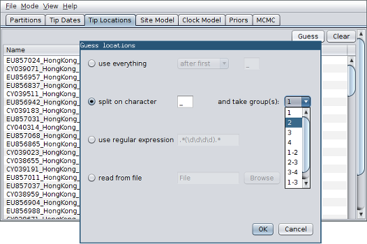
- Click the "Guess" button at the top-right of the panel. This opens the same dialog that we saw in the previous section.
- Because the locations are included as the second element of the underscore-delimited triple in the header, choose the "split on character" radio button and select group 2 from the drop-down menu. (Note again that the underscore character is already chosen as the delimiter.)
After clicking "OK" you should find that the tip location table is populated with locations that match those in the sequence headers, as follows:

For this analysis, we will use the HKY substitution model with base frequencies empirically estimated from the alignment. To configure this in BEAUti:
- Switch to the "Site Model" panel.
- Select HKY from the drop-down menu (the default option is JC69).
- Select "Empirical" from the drop-down menu to the right of the "Frequencies" label.
The BEAUti panel should now look like the following:

Note that the "Substitution rate" defined on this panel should be left unestimated - we use the "Clock rate" defined in the "Clock Model" panel to determine the average per unit time rate of sequence evolution. Used this way, the "substitution rate" is therefore not actually a rate (it's actually dimensionless) but is instead a rate multiplier that in our case we fix at 1.
For this analysis we assume a strict clock. Since our alignment contains sequences sampled at different times and those times are measured in years, we must use a real clock rate expressed in units of expected substitutions per site per year. Usually the precise value is unknown and so the default behaviour of BEAUti is to assume this rate is to be estimated. For this data, however, we happen to know the true value quite well and so we can fix the clock rate to this known value.
To do this, first open the Mode menu and uncheck the "Automatic set clock rate" option:

Then, set the clock rate to 0.005 and uncheck the estimate checkbox. The Clock Model panel should now look like this:

Because the structured coalescent is a model-based prior on the (multi-type) tree distribution, setting up the "Priors" panel is a particularly important part of setting up this analysis.
- Click the arrow to the left of the
structuredCoalescent.t:h3n2_2demeparameter to expand the tree prior. - Ensure the value shown in the "number of demes" spinner is equal to the number of types present in your model. In this case, the default value of 2 is correct, but in general you will need to change this.
- Check the "estimate" checkboxes to the right of the population size vector and migration rate matrix tables. (These tables allow us to modify the initial values of these parameters, or fix them to known values.)
- Use the drop-down menus to change the priors for the
popSizes.t:h3n2andrateMatrix.t:h3n2parameters to "Uniform". - Click the arrows on the left-hand side of each of these parameters to alter the details of these priors, changing the Lower and Upper bounds of the distributions to 0.1 and 3 respectively. (These are very tight priors which we use here to reduce the run time needed for the analysis. You will want to think carefully about the values you use here for any other data.)
With the parameter priors de-expanded, the panel should finally appear as below:

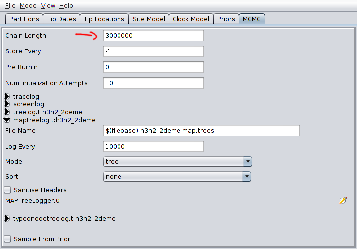
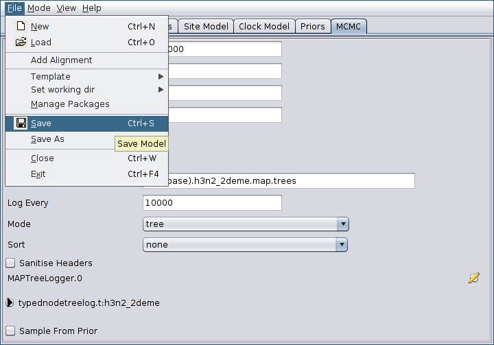
In the MCMC panel, we can adjust the number of steps to use in the MCMC chain that will be used to sample from the joint posterior over multi-type trees and all of the model parameters. In this case, we will reduce the default of 10 million steps down to 3 million steps.
This panel also lets us adjust the fraction of sampled states that are written to the log and tree log files.
Notice that the MultiTypeTree template provides two special log types: the first is "maptreelog". This produces a file containing running estimates of the maximum a posteriori multi-type tree over the course of the analysis. For this particular log type, the sampling period defined in the "Log Every" field also determines the fraction of trees that will be assessed as MAP tree candidates. The default value therefore causes only 1 tree in every 10000 to be considered for this position:
Using smaller sampling periods will improve the accuracy of the MAP estimate at the expense of increased time spent writing trees to disk and increased log file size.
The second MultiTypeTree specific log type is the "typednodetreelog". This records trees in which only the coalescent nodes are annotated with ancestral locations. The log file can be analyzed using TreeAnnotator to produce a summary tree.
At this point we have fully specified our analysis in BEAUti. To actually run it, we need to save the model to an XML file and then run BEAST on that file. To save the model, simply select Save from the File menu:
Using the dialog box, navigate to the directory in which you'd like to keep the analysis files (the desktop, or some tutorial directory for instance). Once this is done, enter a useful filename for the analysis XML file. For this analysis, something like "h3n2_2deme" will suffice. BEAUti will automatically append ".xml" to the file name you specify.
To run the analysis, simply start BEAST 2 in the manner appropriate for your platform, then select the file you generated in the last section as the input file. (Refer to the documentation provided at www.beast2.org for detailed instructions.)
The 3 million steps require on the order of 6 minutes to complete on a modern computer.
If for some reason you have trouble running BEAST on the computer you are using for the tutorial or if anything else goes wrong, you can download the final log files and use them to complete the tutorial.
The results of the analysis primarily consist of two parts:
- The parameter log, which is written to the file
h3n2_2deme.log. - The tree log, which is written to
h3n2_2deme.h3n2_2deme.trees.
In addition, the file h3n2_2deme.h3n2_2deme.map.trees contains the running
estimate of the MAP tree as a function of MCMC step number, while the file
h3n2_2deme.h3n2_2deme.typedNode.trees is the TreeAnnotator-compatible file
we'll use to assemble a summary tree.
We can use the program Tracer to
view the parameter log file. To do this, start Tracer and then press the "+"
button in the top-left hand corner of the window (under "Trace files"). Select
the log file for this analysis (h3n2_2deme.log) from the file selection dialog box.
The "Traces" table will then be populated with parameters and summary
statistics corresponding to our structured coalescent analysis.
Important traces are:
-
migModel.t:h3n2_2deme.popSize_*: These give the (effective) structured coalescent population sizes for each of the locations in your model. -
migModel.t:h3n2_2deme.rateMatrix_A_B: These give the structured coalescent immigration rates from B to A. -
Tree.t:h3n2_2deme.count_A_to_B: these give the actual number of ancestral migrations from location A to location B (backward in time).
The panels tabs at the top-right of the window can be used to display one or more selected traces in various ways. For example, selecting the two population size traces and choosing the "Marginal prob distribution" panel results in the following useful comparison between the sampled population size marginal posterior distributions:
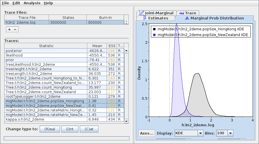
Note that many of the ESS values are still less than 200 - the arbitrary threshold for acceptability. If this analysis were part of a serious study you would want to run the chain for another few million iterations to improve these. (In BEAST 2, analyses can be resumed - the samples you've already acquired will not be wasted.) For the purposes of this tutorial, however, these values are acceptable.
The popular phylogenetic tree visualizer
FigTree can be used to visualize
the sampled trees contained in the tree log h3n2.h3n2.trees and the MAP tree
estimate log h3n2.h3n2.map.trees. Be warned, however, that FigTree currently
takes an extremely long time to load even relatively small (a few megabyte)
MultiTypeTree logs.
For this reasons we suggest using IcyTree to view tree log files and maybe switching to FigTree to visualize summary trees as discussed in the next section. (Also, IcyTree can be used to export individual trees from a large log file for subsequent viewing using FigTree.) IcyTree is a tree viewer that runs in a web browser. It runs best under recent versions of Google Chrome and Mozilla Firefox (in that order).
To view MultiTypeTree log files using IcyTree, simply navigate to the IcyTree web page, select "Load from file" from the "File" menu, then select one of the tree log files using the file selection dialog. Once the file is loaded you will see the first tree it contains. In order to select a different tree, move the mouse pointer over the box in the lower-left corner of the window. This box will expand to a small dialog containing buttons allowing you to navigate between trees. The '<' and '>' buttons move in steps of 1 tree, while '<<' and '>>' move 10% of the tree file per click. You can also directly enter the index of a tree. (Note that there are keyboard shortcuts for almost all commands in IcyTree and that these can be found by selecting "Keyboard shortcuts" from the "Help" menu.)
Initially the trees edges will be uncoloured. To colour the edges according to the edge type, open the "Style" menu, navigate to the "Colour edges by" submenu and select "type". A legend and axis can be added by choosing "Display legend" and "Display axis" from the same menu. Note that the colours are assigned arbitrarily and may be different to those shown in the figures below.
The following shows the final tree of h3n2_2deme.h3n2_2deme.map.log in IcyTree, which
represents our sampled estimate of the MAP multi-type tree:

While IcyTree is useful for rapidly visualizing the results of an analysis, it is not nearly as feature-rich as FigTree and not as capable for producing publication-quality graphics. Happily, however, IcyTree can extract single trees from larger log files. Simply navigate to the desired tree, open the "File" menu, choose the "Export tree as" submenu and select "NEXUS file". (It is important to select "NEXUS" instead of "Newick" as the Newick format does not support the annotations that MultiTypeTree uses to mark the edge types.
While it is tempting to view the MAP tree shown above as the primary result of the phylogenetic side of our analysis it is very important to remember that this is only a point estimate and says nothing about the uncertainty present in the result. This is an important drawback, as we have done a full Bayesian analysis and have access to a large number of samples from the full posterior in the tree log files. The MAP tree discards almost all of this information.
We can make better use of our raw analysis results by using the TreeAnnotator
program which is distributed with BEAST to analyze the
h3n2_2deme.h3n2_2deme.typedNode.trees which were produced by our MCMC run. To do this,
simply load TreeAnnotator and select the h3n2_2deme.h3n2_2deme.typedNode.trees file as
the input file and h3n2_2deme.h3n2_2deme.summary.tree as the output file. Select "Mean
heights" from the "Node heights" menu and set the burn-in percentage to 10:

Pressing the "Run" button will now produce an annotated summary tree.
To visualize this tree, open IcyTree once more (maybe open it in a new browser
tab), choose File->Open, then select the file
h3n2_2deme.h3n2_2deme.summary.tree using the file selection dialog. Follow
the instructions provided for the MAP tree above to colour the tree by the
"type" attribute and add the legend and time axis. In addition, open the Style
menu and from the "Node height error bars" sub-menu select "height_95%_HPD" to
add error bars to the internal node heights. Also, open the Style menu and from
the "Edge opacity" sub-menu select "type.prob". This will cause the edges to
become increasingly transparent as the posterior probability for the displayed
colour decreases.
Once these style preferences have been set, you should see something similar to the following:

Here we have a full consensus tree annotated by the locations at coalescence nodes and showing node height uncertainty, with the widths of the edges representing how certain we can be of the location estimate at each point on the tree. This is a much more comprehensive summary of the phylogenetic side of our analysis.
One thing to pay attention to here is that the most probable root location is
given by the summary tree to be Hong Kong (under our model which assumes that
only Hong Kong and New Zealand exist). By hovering the mouse cursor over the
tiny edge above the root will bring up a table in which posterior probability
of the displayed root location (type.prob) can be seen to be approximately
90%. The analysis therefore strongly supports a Hong Kong origin over a New
Zealand origin. In contrast, the estimated MAP tree gives displays a root
location of NZ. Why is this?
There are at least two answers to this. Firstly, the MAP estimate is a (possibly poor) estimate of the true MAP tree. Secondly, just because the MAP tree has the highest posterior density of any tree sampled, doesn't mean that its individual features are shared with most of the trees sampled.
Over the course of this tutorial we have learned how to
- install the MultiTypeTree package,
- put together a structured coalescent analysis using BEAUti,
- run the analysis using BEAST, and
- process and view the results using Tracer, IcyTree, and TreeAnnotator.
Before finishing, there are three important points that need to be made. The first of these is simply this:
Estimating migration rates is _hard_ - be prepared to wait
a long time for solid results.
This is especially true for models with 4 or more locations/types/demes. In those cases, you will probably want to start thinking about using informative priors on the rate parameters, or at very least setting strict upper (and lower) bounds on the rate parameters.
The second point is this:
Even though it's very tempting, try not to take the MAP tree
estimate too seriously.
This is for the following reasons:
- This is only an estimate of the MAP tree.
- Even the true MAP is only a point estimate. It tells us nothing about the uncertainty associated with any of the migrations/coalescences depicted.
For quantitative purposes it is much better to look only at the marginal distributions of parameters such as those present in the parameter log file. One can also compute additional summary statistics from the tree log file using the TreeLogAnalyser utility that is distributed with BEAST.
The final point is the following:
The summary tree produced by TreeAnnotator ignores migration histories on
the tree edges.
This means that while the movement between types may seem very infrequent on the summary tree, it may in fact be extremely rapid. Thus while the summary tree is a useful picture of our analysis results, it is still important to look at the estimated MAP tree or to browse through the tree log file to get a better picture of what is going on. (Total migration event counts are also recorded in the parameter log file: posterior estimates for those counts give a much better picture of how rapidly individuals in the population are moving around.)