
You can also find all 60 answers here 👉 Devinterview.io - Sorting Algorithms
Sorting algorithms are methods for arranging a dataset in a specific order, such as numerically or alphabetically. They play a critical role in organizing and optimizing data for efficient searching and processing.
-
Comparison-Based Algorithms: Sort elements by comparing them pairwise. Most have
$O(n \log n)$ time complexity. -
Non-Comparison-Based Algorithms: Utilize specialized techniques, often correlated with specific data types. While faster, they are more restricted in their applications.
| Algorithm | Average Case Complexity | Worst Case Complexity | Space Complexity | Stability |
|---|---|---|---|---|
| Bubble Sort | Constant | Yes | ||
| Selection Sort | Constant | No | ||
| Insertion Sort | Constant | Yes | ||
| Merge Sort | Yes | |||
| Quick Sort | In-Place* | No | ||
| Heap Sort | In-Place | No | ||
| Counting Sort | Yes | |||
| Radix Sort | Yes | |||
| Bucket Sort | Yes |
* Note: "In-Place" for Quick Sort means it doesn't require additional space proportional to the input size, but it does require a small amount of extra space for recursive function calls (stack space).
- Trees: Balanced trees (e.g., AVL, Red-Black) use sorted data for efficient operations.
- Heaps: Used in priority queues for quick priority element extraction.
- Graphs: Algorithms like Kruskal's and Dijkstra's benefit from sorted data.
- Indexes: Sorted indices (e.g., B-Trees, B+ Trees) improve database efficiency.
- Feature Analysis: Sorting helps in feature selection and outlier detection.
- Data Cleaning: Sorting aids in deduplication and term frequency analysis.
- Search/Merge:
- Faster searches with binary search on sorted data.
- Parallel merging in distributed systems uses sorted data.
- Visualization: Sorting enhances data representation in charts and histograms.
Sorting algorithms can be categorized based on their characteristics.
-
Comparison-based Algorithms: Rely on comparing the elements to determine their order.
- Examples: QuickSort, Bubble Sort, Merge Sort.
-
Non-comparison based Algorithms: Sort without direct comparisons, often rely on the nature of the data, like the distribution or range of input values.
- Examples: Counting Sort, Radix Sort, Bucket Sort.
-
Hybrid Sorts: Combine the best of both worlds by using quick, comparison-based techniques and then switching to specialized methods when beneficial.
- Examples: IntroSort (combines QuickSort, HeapSort, and Insertion Sort).
-
No or Few Swaps: Designed to minimize the number of swaps, making them efficient for certain types of data.
- Examples: Insertion Sort (optimized for nearly sorted data), QuickSort.
-
Multiple Swaps: Swapping neighboring elements multiple times throughout the sorting process.
- Example: Bubble Sort.
-
Recursive Algorithms: Use a divide-and-conquer approach, breaking the problem into smaller sub-problems and solving them recursively.
- Examples: Merge Sort, QuickSort.
-
Iterative Algorithms: Repeatedly apply a set of operations using loops without making recursive calls.
- Examples: Bubble Sort, Insertion Sort.
-
Stable Algorithms: Elements with equal keys appear in the same order in the sorted output as they appear in the input.
- Examples: Merge Sort, Insertion Sort, Bubble Sort.
-
Unstable Algorithms: The relative order of records with equal keys might change.
- Examples: QuickSort, HeapSort, Selection Sort.
-
Adaptive Algorithms: Take advantage of existing order in the dataset, meaning their performance improves when dealing with partially sorted data or data that has some inherent ordering properties.
- Examples: Insertion Sort, Bubble Sort, IntroSort.
-
Non-Adaptive Algorithms: Performance remains the same regardless of the initial order of the dataset.
- Examples: Merge Sort, HeapSort.
-
In-Place Algorithms: Sort the input data within the same space where it's stored, using only a constant amount of extra memory (excluding the call stack in the case of recursive algorithms).
- Examples: QuickSort, Bubble Sort, Insertion Sort.
-
Not-In-Place Algorithms: Require additional memory or data structures to store temporary data.
- Examples: Merge Sort, Counting Sort.
| Algorithm | Method | In-Place | Adaptive | Stability | Swaps / Inversions | Recursion vs. Iteration |
|---|---|---|---|---|---|---|
| QuickSort | Divide and Conquer | Yes* | No* | Unstable | Few | Recursive |
| Bubble Sort | Exchange | Yes | Yes | Stable | Multiple | Iterative |
| Merge Sort | Divide and Conquer | No | No | Stable | - | Recursive |
| Counting Sort | Non-comparative | No | No | Stable | - | Iterative |
| Radix Sort | Non-comparative | No | No | Stable | - | Iterative |
| Bucket Sort | Distributive | No | No | Depends* | - | Iterative |
| IntroSort | Hybrid | Yes | No | Unstable | Few | Recursive and Iterative |
| Insertion Sort | Incremental | Yes | Yes | Stable | Few | Iterative |
| HeapSort | Selection | Yes | No | Unstable | - | Iterative |
* Notes:
- QuickSort: Depending on implementation, can be in-place or not, and can be adaptive or not.
- Bucket Sort: Stability depends on the sorting algorithm used within each bucket.
An ideal sorting algorithm would have these key characteristics:
- Stability: Maintains relative order of equivalent elements.
- In-Place Sorting: Minimizes memory usage.
- . Adaptivity: Adjusts strategy based on data characteristics.
-
Time Complexity: Ideally
$O(n \log n)$ for comparisons. -
Space Complexity: Ideally
$O(1)$ for in-place algorithms. - Ease of Implementation: It should be straightforward to code and maintain.
While no single algorithm perfectly matches all the ideal criteria, some come notably close:
Timsort, a hybrid of Merge Sort and Insertion Sort, is designed for real-world data, being adaptive, stable, and having a consistent
HeapSort offers in-place sorting with
Divide and Conquer is a fundamental algorithm design technique that breaks a problem into smaller, more manageable sub-problems, solves each sub-problem separately, and then combines the solutions to the sub-problems to form the solution to the original problem.
- Divide: The original problem is divided into a small number of similar sub-problems.
- Conquer: The sub-problems are solved recursively. If the sub-problems are small enough, their solutions are straightforward, and this stopping condition is called the "base case".
- Combine: The solutions to the sub-problems are then combined to offer the solution to the original problem.
Many well-known sorting algorithms, such as Quick Sort, Merge Sort, and Heap Sort, use this strategy.
-
Efficiency: These algorithms often outperform simpler algorithms in practice, and can have
$O(n \log n)$ worst-case time complexity. -
Parallelism: Divide and Conquer algorithms are amenable to parallelization, promoting parallel processing.
-
Memory Access: Their memory access patterns often result in better cache performance.
These algorithms are integral in various computing systems, ranging from general-purpose systems to specialized uses, where they contribute to faster and more efficient operations.
Here is the Python code:
def merge_sort(arr):
    if len(arr) > 1:
        mid = len(arr) // 2  # Run-time: O(1)
        left = arr[:mid]  # Run-time: O(n)
        right = arr[mid:]  # Run-time: O(n)

        merge_sort(left)  # T(n/2) - Both left and right sub-arrays will be half of the original array
        merge_sort(right)  # T(n/2)

        merge(arr, left, right)  # O(n)

def merge(arr, left, right):
    i = j = k = 0

    while i < len(left) and j < len(right):
        if left[i] < right[j]:
            arr[k] = left[i]
            i += 1
        else:
            arr[k] = right[j]
            j += 1
        k += 1

    while i < len(left):
        arr[k] = left[i]
        i += 1
        k += 1

    while j < len(right):
        arr[k] = right[j]
        j += 1
        k += 1
Time Complexity:
The time complexity for Merge Sort can be expressed with the recurrence relation:
which solves to
Let's look at the fundamental differences between comparison-based and non-comparison-based sorting algorithms.
-
Non-comparison based algorithms: Algorithms such as radix sort and counting sort do not rely on direct element-by-element comparisons to sort items. Instead, they exploit specific properties of the data, often making them more efficient than comparison-based sorts in these special cases.
-
Comparison-based algorithms: These algorithms, including quick sort, merge sort, and heap sort, use direct comparisons to establish the sorted order. The focus is on ensuring that every element is compared to all others as needed.
-
Non-comparison based algorithms may sometimes achieve better time and/or space complexities. For example, counting sort can achieve a time complexity of
$O(n + k)$ and a space complexity of$O(n + k)$ , where$k$ represents the range of numbers in the input array. This is due to its characteristic of not performing comparisons. -
Comparison-based algorithms, by nature of requiring element-to-element comparisons, generally achieve at least
$O(n \log n)$ time complexity (for worst-case or average-case scenarios, in many cases). The space complexity can vary but is often$O(n)$ , especially when using recursive techniques.
-
Stable sorts: Some sorting algorithms can preserve the original order of equal elements in the sorted output, ensuring that earlier occurrences of equal elements appear before later ones. For instance, merge sort, bubble sort, and insertion sort are typically stable sorts.
-
Unstable sorts: These algorithms cannot guarantee the preservation of original order. Even though most modern quicksort implementations use techniques to ensure stability, in general, quicksort is considered unstable.
-
Comparison-based nature: Selection sort works by repeatedly selecting the minimum remaining element and swapping it with the first unsorted element, making direct comparisons each time.
-
Non-comparison examples: Selection sort is a straightforward algorithm where you directly compare elements to find the minimum. It's always preferred to use sorting algorithms that are more efficient and might take advantage of specific characteristics of the data.
In-Place sorting refers to algorithms that rearrange data within its existing storage, without needing extra memory for the sorted result.
This is especially useful in limited-memory situations. In most cases, it allows for faster sort operations by avoiding costly data movement between data structures.
- QuickSort
- HeapSort
- BubbleSort
- Insertion Sort
- Selection Sort
- Dual-Pivot QuickSort
- Introselect (or Introspective Sort)
When it comes to sorting algorithms, there is a distinction between stable and unstable algorithms.
A "stable algorithm" leaves items with equal keys in the same relative order they had before sorting. This characteristic can be crucial in certain cases.
Conversely, an "unstable algorithm" makes no guarantees about the original order of items with equal keys.
Consider a list of students, their scores, and the date they took the test:
| Name | Score | Date |
|---|---|---|
| Alice | 85 | 2023-01-05 |
| Bob | 85 | 2023-01-03 |
| Charlie | 80 | 2023-01-04 |
| David | 90 | 2023-01-02 |
If we sort this list by score using a stable sort algorithm, the result would be:
| Name | Score | Date |
|---|---|---|
| Charlie | 80 | 2023-01-04 |
| Bob | 85 | 2023-01-03 |
| Alice | 85 | 2023-01-05 |
| David | 90 | 2023-01-02 |
Note that both Bob and Alice have a score of 85, but Bob is listed before Alice in the result because he took the test before her.
However, if we sorted the same list by score using an unstable sorting algorithm, the result could be:
| Name | Score | Date |
|---|---|---|
| Charlie | 80 | 2023-01-04 |
| Alice | 85 | 2023-01-05 |
| Bob | 85 | 2023-01-03 |
| David | 90 | 2023-01-02 |
Here, Alice is listed before Bob despite having taken the test later. The relative order based on the test date is not preserved for records with equal scores, which illustrates the behavior of an unstable sorting algorithm.
External sorting is designed to efficiently handle large datasets that can't fit entirely in system memory. It accomplishes this by using a combination of disk storage and memory.
In contrast, internal sorting methods are suitable for small to modest datasets that can fit entirely in memory, making them faster and simpler to operate.
- External: Utilizes both system memory and disk space.
- Internal: Functions solely within system memory.
- External: Algorithm's execution time can depend on data access from disk storage.
- Internal: Generally faster due to the absence of disk access overhead.
- External: Splits data among multiple storage units, typically using primary memory as the main sorting area.
- Internal: Works directly on the entire dataset present in memory.
- External Merge Sort
- Polyphase Merge Sort
- Replacement Selection
- Distribution Sort
- Bubble Sort
- Insertion Sort
- Selection Sort
- QuickSort
- Merge Sort
- HeapSort
- Radix Sort
- Counting Sort
Here is the Python code:
def quicksort(arr):
    if len(arr) <= 1:
        return arr
    pivot = arr[len(arr) // 2]
    left = [x for x in arr if x < pivot]
    middle = [x for x in arr if x == pivot]
    right = [x for x in arr if x > pivot]
    return quicksort(left) + middle + quicksort(right)

# Example usage
my_list = [3, 6, 8, 10, 1, 2, 1]
print(quicksort(my_list)) # Output: [1, 1, 2, 3, 6, 8, 10]Here is the Python code:
def external_merge_sort(input_file, output_file, memory_limit):
    split_files = split_file(input_file, memory_limit)
    sorted_files = [sort_file(f) for f in split_files]
    merge_files(sorted_files, output_file)

def split_file(input_file, memory_limit):
    # Split the input file into smaller chunks that fit in memory
    # Return a list of filenames of the chunks

def sort_file(filename):
    # Load the file into memory, sort it using a method like QuickSort, and save back to disk
    # Return the filename of the sorted chunk

def merge_files(sorted_files, output_file):
    # Implement a k-way merge algorithm to merge the sorted files into a single output file

# Example usage
external_merge_sort("large_dataset.txt", "sorted_dataset.txt", 1000000)Adaptive sorting algorithms are tailored to take advantage of a dataset's existing order. When data is partially sorted, adaptive algorithms can be faster than non-adaptive ones.
- Memory Efficiency: They often use less memory than non-adaptive algorithms.
- Operator Type: Can be stable, but stability is not guaranteed in all circumstances. Stability ensures that relative order of equal elements remains the same.
- Performance: Their core defining feature is that they use information about the data to speed up the sorting process.
-
Insertion Sort: Efficient on small datasets and partially sorted data. Its best and average case time complexities reduce drastically in the presence of order, making it adaptive.
-
Bubble Sort/Selection Sort: Though generally non-adaptive, certain optimized forms can exhibit adaptivity for specific use-cases.
-
QuickSort: Can be adaptive when carefully implemented. If done so, it witnesses a performance boost with partially sorted datasets.
-
Merge Sort: Known for its deterministic and consistent behavior, it is generally non-adaptive. However, there exist hybrid versions that adapt to specific conditions, such as the "TimSort" algorithm used in Python and Java.
Here is the Python code:
def insertion_sort(arr):
for i in range(1, len(arr)):
key = arr[i]
j = i - 1
while j >= 0 and arr[j] > key:
arr[j + 1] = arr[j]
j -= 1
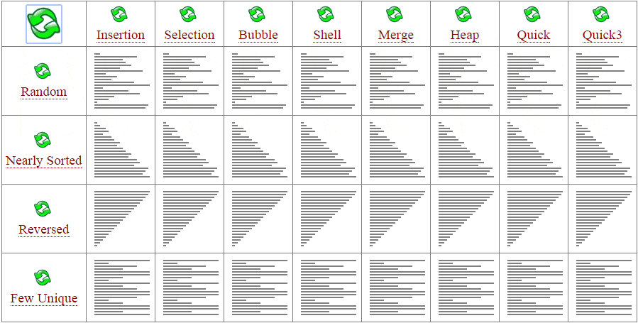
arr[j + 1] = key10. How does the Time Complexity of sorting algorithms change with respect to Different Types of Input Data?
Knowing how sorting time complexity changes based on input data empowers you to choose the most effective algorithm.
The performance of sorting algorithms depends on the initial distribution state of the elements, such as whether the dataset is already partially sorted or consists of distinct values. Let's delve into the unique characteristics of specific sorting methods for varying input types:
-
Best-Case (Fewest Operations): When the list or array is already sorted or near-sorted, time complexity is minimized:
- Bubble, Selection, and Insertion Sort:
$O(n)$ - Merge Sort:
$O(n \log n)$ - Quick Sort:
$O(n \log n)$ with the best pivot selection, which is achieved with certain methods like "median of three" to ensure a balanced division.
- Bubble, Selection, and Insertion Sort:
-
Worst-Case (Most Operations): Indicates the highest number of operations required to sort the dataset. Algorithms are optimized to minimize this in various ways:
- Bubble Sort:
$O(n^2)$ when the list is in reverse order, and Bubble Sort does$n - 1$ passes. - Selection Sort:
$O(n^2)$ regardless of the input data, as it makes the same number of comparisons in all cases and performs$n - 1$ exchanges, even when the list is already sorted. - Insertion Sort:
$O(n^2)$ when the list is in reverse order. It performs best when the list is almost sorted and requires only$O(n)$ operations.
- Bubble Sort:
-
Average-Case (Balanced Scenario): Considers the dataset's behavior in an average state, taking into account all possible permutations:
- Bubble Sort:
$O(n^2)$ - Selection Sort:
$O(n^2)$ - Insertion Sort:
$O(n^2)$ typically (can be$O(n)$ for almost sorted data). - Merge Sort:
$O(n \log n)$ - Quick Sort:
$O(n \log n)$
- Bubble Sort:
-
Adaptive Algorithms: Vary Based on Input Characteristics:
- Algorithms like Insertion Sort and Bubble Sort adapt to the dataset's characteristics during execution. If the dataset is almost sorted, they perform fewer operations:
- Insertion Sort:
$O(k + n)$ where$k$ is the number of inversions and$n$ is the number of elements. - Bubble Sort: Can be as low as
$O(n)$ in the best case with almost-sorted data.
- Insertion Sort:
- Algorithms like Insertion Sort and Bubble Sort adapt to the dataset's characteristics during execution. If the dataset is almost sorted, they perform fewer operations:
-
External Memory (Secondary Storage Devices): For vast datasets where elements can't fit into primary memory, merge-sort based algorithms (like K-way merge) are the most suitable. Their time complexity is dominantly influenced by the number of external passes needed and the internal sorting within the allocated memory, leading to an overall time complexity of
$O(\text{{number of records}} \cdot \log_{\text{{M}}}( \text{{number of records}} / \text{{M}}))$ where$M$ is the number of records that can be sorted in internal memory.
For the in-place sorting algorithms (like quicksort), they need to be carefully chosen for nearly sorted datasets, where they might still perform well.
- Stable sorting algorithms retain the relative order of equal elements. For instance, in a list of students sorted first by name and then by GPA, the stable algorithm ensures that students with the same name remain ordered by their GPAs.
- Unstable sorting algorithms do not guarantee the maintenance of relative order for equal elements.
-
Cycle Detection Algorithms: The CLEAD algorithm is employed in Timsort for cycle detection, enabling worst-case time complexity of
$O(n \log n)$ and making it practical even for real-world data with recurring patterns or cycles. -
Adaptive Algorithms: These adjust their strategies based on the characteristics of the dataset.
- Algorithms like Quick Sort, designed originally as non-adaptive, can be refined using techniques like "median of three" for enhanced adaptiveness for real-world datasets.
- The Introsort algorithm blends quicksort and heap sort, starting with quicksort and transitioning to heapsort if the recursion depth surpasses a certain threshold.
- Comparison-Counting: Some algorithms, such as heapsort, rely on a constant number of comparisons at each step, making them more predictable in their time complexity evaluations.
Bubble Sort is a basic and often inefficient sorting algorithm. It continually compares adjacent elements and swaps them until the list is sorted.
- Comparison-Based: Sorts elements based on pairwise comparisons.
- Adaptive: Performs better on partially sorted data.
- Stable: Maintains the order of equal elements.
-
In-Place: Requires no additional memory, with a constant space complexity of
$O(1)$ .
-
Inefficient for Large Datasets: Bubble Sort has a worst-case and average-case time complexity of
$O(n^2)$ , making it unsuitable for large datasets. - Lacks Parallelism: Its design makes it difficult to implement in parallel computing architectures.
- Suboptimal for Most Scenarios: With quadratic time complexity and numerous better alternatives, Bubble Sort generally isn't a practical choice in production.
- Flag Setup: Initialize a flag to track if any swaps occur in a pass.
- Iterative Pass: Starting from the first element, compare neighboring elements and swap them if necessary. Set the flag if a swap occurs.
- Early Termination: If a pass doesn't result in any swaps, the list is sorted, and the algorithm stops.
- Repetitive Passes: Complete additional passes if needed.

-
Time Complexity:
- Best Case:
$O(n)$ - When the list is already sorted and no swaps occur. - Worst and Average Case:
$O(n^2)$ - When every element requires multiple swaps to reach its correct position.
- Best Case:
-
Space Complexity:
$O(1)$
Here is the Python code:
def bubble_sort(arr):
    n = len(arr)
    for i in range(n - 1):
        for j in range(n - i - 1):
            if arr[j] > arr[j + 1]:
                arr[j], arr[j + 1] = arr[j + 1], arr[j]
return arrBubble Sort, while not the most efficient, can benefit from several performance-enhancing modifications.
Improved Efficiency: Reduces the number of passes through the list.
For small or nearly sorted arrays, terminating the sorting process early when an iteration has no swaps can make the algorithm nearly linear (
Improved Efficiency: Reduces the number of comparisons in subsequent iterations.
By restricting the inner loop to the position of the last swap, redundant comparisons are minimized, especially beneficial for lists that become partially sorted early on.
Improved Efficiency: Reduces "turtle" items (small items towards the end) which Bubble Sort is typically slow to move.
This variant alternates between forward and backward passes through the list, helping to move both large and small out-of-place elements more rapidly.
Improved Efficiency: Speeds up the sorting of smaller elements at the list's beginning.
Inspired by Bubble Sort, Comb Sort uses a gap between compared elements that reduces each iteration. This adjustment can make the algorithm faster than traditional Bubble Sort, especially for long lists.
Improved Efficiency: Can lead to faster convergence for certain datasets.
A variation where pairs of adjacent elements are compared iteratively, first with an odd index and then an even index, and vice versa in subsequent passes. Its parallelizable nature can lead to efficiency improvements on multi-core systems.
Here is the Python code:
def bubble_sort(arr):
    is_sorted = False
    last_swap = len(arr) - 1
    while not is_sorted:
        is_sorted = True
        new_last_swap = 0
        for i in range(last_swap):
            if arr[i] > arr[i + 1]:
                arr[i], arr[i + 1] = arr[i + 1], arr[i]
                is_sorted = False
                new_last_swap = i
        last_swap = new_last_swap

        if is_sorted:
            break
return arrInsertion Sort is a straightforward and intuitive sorting algorithm that builds the final sorted array one element at a time. It's similar to how one might sort a hand of playing cards.
- Comparison-Based: Uses pairwise comparisons to determine the correct position of each element.
- Adaptive: Performs more efficiently with partially sorted data, offering near-linear time for such scenarios.
- Stable: Preserves the order of equal elements.
- In-Place: Operates directly on the input data, using a minimal constant amount of extra memory space.
-
Not Ideal for Large Datasets: With a worst-case and average-case time complexity of
$O(n^2)$ , Insertion Sort isn't the best choice for large lists. - Simplistic Nature: While easy to understand and implement, it doesn't offer the advanced optimizations present in more sophisticated algorithms.
- Outperformed in Many Cases: More advanced algorithms, such as QuickSort or MergeSort, generally outperform Insertion Sort in real-world scenarios.
- Initialization: Consider the first element to be sorted and the rest to form an unsorted segment.
- Iterative Expansion: For each unsorted element, 'insert' it into its correct position in the already sorted segment.
- Position Finding: Compare the current element to the previous elements. If the current element is smaller, it is shifted to the left until its correct position is found.
- Completion: Repeat the process for each of the elements in the unsorted segment.

-
Time Complexity:
- Best Case:
$O(n)$ - When the input list is already sorted. - Worst and Average Case:
$O(n^2)$ - Especially when the input is in reverse order.
- Best Case:
-
Space Complexity:
$O(1)$
Here is the Python code:
def insertion_sort(arr):
    for i in range(1, len(arr)):
        key = arr[i]
        j = i - 1
        while j >= 0 and key < arr[j]:
            arr[j + 1] = arr[j]
            j -= 1
        arr[j + 1] = key
return arrMerge Sort is a robust and efficient divide-and-conquer sorting algorithm. It breaks down a list into numerous sublists until each sublist consists of a single element and then merges these sublists in a sorted manner.
- Divide and Conquer: Segments the list recursively into halves until individual elements are achieved.
- Stable: Maintains the order of equal elements.
-
External: Requires additional memory space, leading to a linear space complexity
$O(n)$ . - Non-Adaptive: Does not benefit from existing order in a dataset.
-
Consistent Performance: Merge Sort guarantees a time complexity of
$O(n \log n)$ across best, average, and worst-case scenarios. - Parallelizable: Its design allows for efficient parallelization in multi-core systems.
-
Widely Used: Due to its reliable performance, it's employed in many systems, including the
sort()function in some programming languages.
- Divide: If the list has more than one element, split the list into two halves.
- Conquer: Recursively sort both halves.
- Merge: Combine (merge) the sorted halves to produce a single sorted list.
-
Time Complexity: Best, Average, and Worst Case:
$O(n \log n)$ - Due to the consistent halving and merging process. -
Space Complexity:
$O(n)$ - Additional space is required for the merging process.
Here is the Python code:
def merge_sort(arr):
    if len(arr) > 1:
        mid = len(arr) // 2
        left = arr[:mid]
        right = arr[mid:]

        merge_sort(left)
        merge_sort(right)

        i = j = k = 0

        while i < len(left) and j < len(right):
            if left[i] < right[j]:
                arr[k] = left[i]
                i += 1
            else:
                arr[k] = right[j]
                j += 1
            k += 1

        while i < len(left):
            arr[k] = left[i]
            i += 1
            k += 1

        while j < len(right):
            arr[k] = right[j]
            j += 1
            k += 1

return arrQuickSort is a highly efficient divide-and-conquer sorting algorithm that partitions an array into subarrays using a pivot element, separating elements less than and greater than the pivot.
- Divide and Conquer: Uses a pivot to partition the array into two parts and then sorts them independently.
-
In-Place: Requires minimal additional memory, having a space complexity of
$O(\log n)$ due to recursive call stack. - Unstable: Does not maintain the relative order of equal elements.
- Versatile: Can be tweaked for better performance in real-world situations.
- Cache-Friendly: Often exhibits good cache performance due to its in-place nature.
- Parallelizable: Its divide-and-conquer nature allows for efficient parallelization in multi-core systems.
-
Worst-Case Performance: QuickSort has a worst-case time complexity of
$O(n^2)$ , although this behavior is rare, especially with good pivot selection strategies.
- Pivot Selection: Choose an element from the array as the pivot.
- Partitioning: Reorder the array so that all elements smaller than the pivot come before, while all elements greater come after it. The pivot is then in its sorted position.
- Recursive Sort: Recursively apply the above steps to the two sub-arrays (elements smaller than the pivot and elements greater than the pivot).
-
Time Complexity:
- Best and Average Case:
$O(n \log n)$ - When the partition process divides the array evenly. - Worst Case:
$O(n^2)$ - When the partition process divides the array into one element and$n-1$ elements, typically when the list is already sorted.
- Best and Average Case:
-
Space Complexity:
$O(\log n)$ - Due to the recursive call stack.
Here is the Python code:
def quick_sort(arr):
    if len(arr) <= 1:
        return arr
    pivot = arr[len(arr) // 2]
    left = [x for x in arr if x < pivot]
    middle = [x for x in arr if x == pivot]
    right = [x for x in arr if x > pivot]
    return quick_sort(left) + middle + quick_sort(right)
Explore all 60 answers here 👉 Devinterview.io - Sorting Algorithms