Representation Learning, Manifold Learning and Metric Learning are about how to learn the intrinsic structure of data.
The objective of representation and metric learning is to build new spaces of representations to improve the performance of a classification, regression or clustering algorithm either from distance constraints or by making use of fine decomposition of instances in complete samples.
Manifold learning and finding low-dimensional structure in data is an important task.

- Representation Learning: A Review and New Perspectives
- Symbolic Representation Learning
- Representation Learning on Networks
- Representation learning in graph and manifold
- Learning and Reasoning with Graph-Structured Representations, ICML 2019 Workshop
- Relational Representation Learning
- Scene Graph Representation and Learning
- MINE — Mutual Information Neural Estimation
- An Overview on Data Representation Learning: From Traditional Feature Learning to Recent Deep Learning
- 4th Workshop on Representation Learning for NLP
- Workshop on Representation Learning for Complex
- 1st International Workshop on Graph Representation Learning and its Applications
- Representation Learning :600.479/679 Fall 2014
- Representation Learning 600.479 Fall 2016
- Representation Learning on Graphs: Methods and Applications
- DOOCN-XII: Network Representation Learning Dynamics On and Of Complex Networks 2019
- Representation learning: a unified deep learning framework for automatic prostate MR segmentation
- Representation Learning Mar. 27 – Mar. 31, 2017@simons.berkeley.edu
- Deep Learning and Representation Learning
- Robustness beyond Security: Representation Learning
- ACL Special Interest Group on Representation Learning
- CSC 2414H: Metric Embeddings
- CS294-158 Deep Unsupervised Learning Spring 2019
- Deep Unsupervised Learning NUS SoC, 2019/2020, Semester I
- Neural Discrete Representation Learning
- Representation Learning
- BIGDATA: Collaborative Research: F: Stochastic Approximation for Subspace and Multiview Representation Learning
- CRII: III: Scaling up Distance Metric Learning for Large-scale Ultrahigh-dimensional Data
- https://www.cs.cmu.edu/~anupamg/adv-approx/lecture20.pdf
- https://mnick.github.io/project/geometric-representation-learning/
- CS 227: Knowledge Representation and Reasoning
- What is a Knowledge Representation?
- Why Knowledge Representation Matters
- CSE 4/563: Knowledge Representation: Stuart C. Shapiro
- http://binaryanalysisplatform.github.io/
- http://frankchu.tech/2018/10/08/kr-summary/
- https://github.com/shaoxiongji/awesome-knowledge-graph
- https://kgtutorial.github.io/
- https://kg4ir.github.io/
- https://scientific-knowledge.github.io
- http://geneontology.org/search.html
- KGMA 2019
- COIN: COmmonsense INference in Natural Language Processing
- Vampire: Automatic theorem proving
- https://52paper.github.io/
- https://adityasomak.github.io/
- https://uniformal.github.io/doc/
- https://tyliupku.github.io/
- https://ermongroup.github.io/cs323-notes/logic/representation/
- Second International Workshop on Capturing Scientific Knowledge
- https://xmhe.bitbucket.io/
- http://paperreading.club/
- https://ai-distillery.io/
- https://amds123.github.io/
- http://jalammar.github.io/
- Network Embedding
- 如何评价百度新发布的NLP预训练模型ERNIE? - 知乎
- Jure Leskovec.
- http://www-connex.lip6.fr/~denoyer/wordpress/
- https://blog.feedly.com/learning-context-with-item2vec/
- Six mathematical gems from the history of Distance Geometry
- LOW-DISTORTION EMBEDDINGS OF FINITE METRIC SPACES
- On Certain Metric Spaces Arising From Euclidean Spaces by a Change of Metric and Their Imbedding in Hilbert Space

- http://www.glottopedia.org/index.php/Semantic_representation
- semantic matching in information retrieval
- Semantic Web
- visual semantic embedding
- SEMBED: Semantic Embedding of Egocentric Action Videos
- Latent Semantic Representation Learning for Scene Classification
- Improving Visual Semantic Embedding By Adversarial Contrastive Estimation
- Semantic trees for training word embeddings with hierarchical softmax
- ''Analogies Explained'' ... Explained
- Deep Embedding Logistic Regression
- DeViSE: A Deep Visual-Semantic Embedding Model
- Deep Visual-Semantic Alignments for Generating Image Descriptions
- Semantic Embedding for Sketch-Based 3D Shape Retrieval
- A Dual Attention Network with Semantic Embedding for Few-shot Learning
- Semantic AI: Bringing Machine Learning and Knowledge Graphs Together
- https://2018.eswc-conferences.org/
- The State of the Art in Semantic Representation
- https://cs.nyu.edu/courses/spring10/G22.2590-001/Lecture11.html
- Deep Semantic Embedding
- Learning Deep Structured Semantic Models for Web Search using Clickthrough Data
- Siamese LSTM for Semantic Similarity Analysis
- Deep Learning Embedding/
- Deep Structural Network Embedding (KDD 2016) in Keras Dec. 16th 2017
- Deep Learning of Knowledge Graph Embeddings for Semantic Parsing of Twitter Dialogs
- Knowledge Graph Embeddings
- Knowledge Graph Embedding: A Survey of Approaches and Applications
- Must-read papers on knowledge representation learning (KRL) / knowledge embedding (KE)
- Probabilistic Knowledge Graph Embeddings
- Knowledge Graph Embeddings with node2vec for Item Recommendation
- https://www.cntk.ai/pythondocs/index.html
- https://allenai.github.io/allennlp-docs/index.html
- https://lidchallenge.github.io/
- https://wabyking.github.io/talks/
- http://mostafadehghani.com/
- http://ruder.io/word-embeddings-2017/
- http://xiaohan2012.github.io/articles/
- Simple and efficient semantic embeddings for rare words, n-grams, and language features
- Learning Word Embedding
- Arithmetic Properties of Word Embeddings
- Word Embedding Models
- Embeddings, NN, Deep Learning, Distributional Semantics … in NLP
In natural language processing, the word can be regarded as the node in a graph, which only takes the relation of locality or context.
It is difficult to learn the concepts or the meaning of words. The word embedding technique word2vec maps the words to fixed length real vectors:
$$
f: \mathbb{W}\to\mathbb{V}^d\subset \mathbb{R}^d.
$$
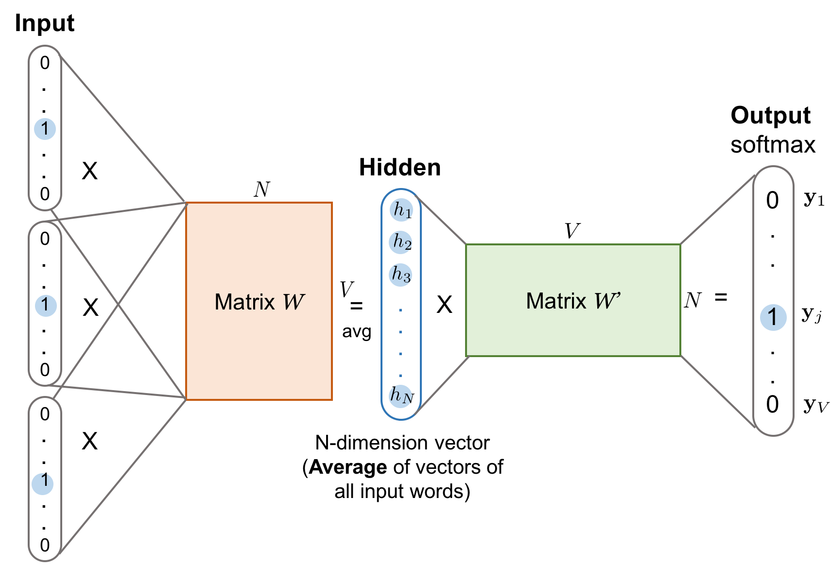
The skip-gram model assumes that a word can be used to generate the words that surround it in a text sequence.
We assume that, given the central target word, the context words are generated independently of each other.
The conditional probability of generating the context word for the given central target word can be obtained by performing a softmax operation on the vector inner product: $$ P(w_o|w_c) = \frac{\exp(u_o^T u_c)}{\sum_{i\in\mathbb{V}} \exp(u_i^T u_c)}, $$
where vocabulary index set
Here, any time step that is less than 1 or greater than
The skip-gram model parameters are the central target word vector and context word vector for each individual word. In the training process, we are going to learn the model parameters by maximizing the likelihood function, which is also known as maximum likelihood estimation. his is equivalent to minimizing the following loss function: $$ -\log(\prod_{t=1}^{T}\prod_{-m\leq j \leq m, j\not = i}{P}(w^{(t+j)}\mid w^{(j)})) = \ -\sum_{t=1}^{T}\sum_{-m\leq j \leq m, j \not= i} \log({P}(w^{(t+j)}|w^{(j)}))). $$
And we could compute the negative logarithm of the conditional probability $$ -\log(P(w_o|w_c)) = -\log(\frac{\exp(u_o^T u_c)}{\sum_{i\in\mathbb{V}} \exp(u_i^T u_c)}) \= -u_o^T u_c + \log(\sum_{i\in\mathbb{V}} \exp(u_i^T u_c)). $$
Then we could compute the gradient or Hessian matrix of the loss functions to update the parameters such as:
The continuous bag of words (CBOW) model is similar to the skip-gram model. The biggest difference is that the CBOW model assumes that the central target word is generated based on the context words before and after it in the text sequence. Let central target word
$$
P(w_c|w_{o_1},\cdots, w_{o_{2m}}) = \frac{\exp(\frac{1}{2m}u_c^T(u_{o_1}+ \cdots + u_{o_{2m}}))}{\sum_{i\in V}\exp(\frac{1}{2m} u_i^T(u_{o_1}+ \cdots + u_{o_{2m}}))}.
$$
hierarchical softmax, negative sample
- https://code.google.com/archive/p/word2vec/
- https://skymind.ai/wiki/word2vec
- https://arxiv.org/abs/1402.3722v1
- https://zhuanlan.zhihu.com/p/35500923
- https://zhuanlan.zhihu.com/p/26306795
- https://zhuanlan.zhihu.com/p/56382372
- http://anotherdatum.com/vae-moe.html
- https://d2l.ai/chapter_natural-language-processing/word2vec.html
- https://www.gavagai.io/text-analytics/word-embeddings/
- http://jalammar.github.io/illustrated-word2vec/
- https://devmount.github.io/GermanWordEmbeddings/
- Contextual String Embeddings for Sequence Labeling
- https://blog.csdn.net/Walker_Hao/article/details/78995591
- Distributed Representations of Sentences and Documents
- Sentiment Analysis using Doc2Vec
- From Word Embeddings To Document Distances
- Learning and Reasoning with Graph-Structured Representations, ICML 2019 Workshop
- Statistical Models of Language
- Semantic Word Embeddings
- Word Embeddings
- GloVe: Global Vectors for Word Representation Jeffrey Pennington, Richard Socher, Christopher D. Manning
- Word embedding
- Open Sourcing BERT: State-of-the-Art Pre-training for Natural Language Processing? Friday, November 2, 2018
- Deep Semantic Embedding
- 无监督词向量/句向量?:W2v/Glove/Swivel/ELMo/BERT
- The Expressive Power of Word Embeddings
- word vector and semantic similarity
- Entity Embeddings of Categorical Variables
- https://mc.ai/entity-embedding/
- https://github.com/dkn22/embedder
- https://tidymodels.github.io/embed/index.html
Gradient Boosted Categorical Embedding and Numerical Trees (GB-CSENT) is to combine Tree-based Models and Matrix-based Embedding Models in order to handle numerical features and large-cardinality categorical features.
A prediction is based on:
- Bias terms from each categorical feature.
- Dot-product of embedding features of two categorical features,e.g., user-side v.s. item-side.
- Per-categorical decision trees based on numerical features ensemble of numerical decision trees where each tree is based on one categorical feature.
In details, it is as following: $$ \hat{y}(x) = \underbrace{\underbrace{\sum_{i=0}^{k} w_{a_i}}{bias} + \underbrace{(\sum{a_i\in U(a)} Q_{a_i})^{T}(\sum_{a_i\in I(a)} Q_{a_i}) }{factors}}{CAT-E} + \underbrace{\sum_{i=0}^{k} T_{a_i}(b)}_{CAT-NT}. $$ And it is decomposed as the following table.
| Ingredients | Formulae | Features |
|---|---|---|
| Factorization Machines | $\underbrace{\underbrace{\sum_{i=0}^{k} w_{a_i}}{bias} + \underbrace{(\sum{a_i\in U(a)} Q_{a_i})^{T}(\sum_{a_i\in I(a)} Q_{a_i}) }{factors}}{CAT-E}$ | Categorical Features |
| GBDT | Numerical Features |
- http://www.hongliangjie.com/talks/GB-CENT_Boston_2017-09-07.pdf
- Talk: Gradient Boosted Categorical Embedding and Numerical Trees
- Paper: Gradient Boosted Categorical Embedding and Numerical Trees
- https://qzhao2018.github.io/zhao/
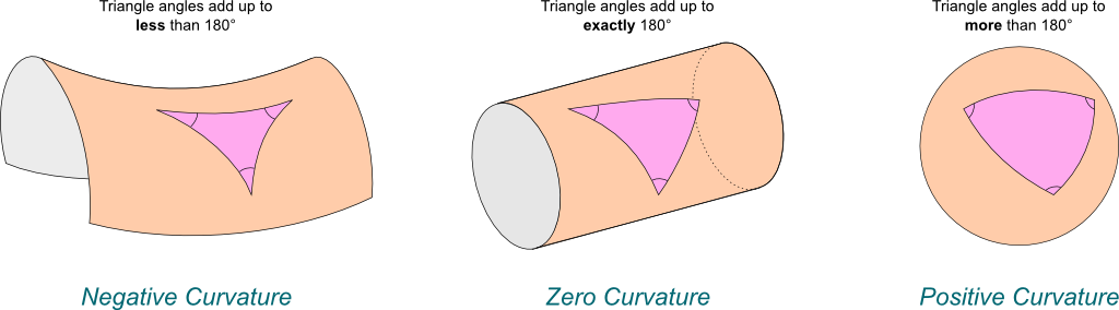
The motivation of hyperbolic embedding is to combine structural information with continuous representations suitable for machine learning methods. One example is embedding taxonomies (such as Wikipedia categories, lexical databases like WordNet, and phylogenetic relations).
The big goal when embedding a space into another is to preserve distances and more complex relationships. It turns out that hyperbolic space can better embed graphs (particularly hierarchical graphs like trees) than is possible in Euclidean space. Even better—angles in the hyperbolic world are the same as in Euclidean space, suggesting that hyperbolic embeddings are useful for downstream applications (and not just a quirky theoretical idea).
The motivation is to embed structured, discrete objects such as knowledge graphs into a continuous representation that can be used with modern machine learning methods. Hyperbolic embeddings can preserve graph distances and complex relationships in very few dimensions, particularly for hierarchical graphs.
Hyperbolic Axiom: There is a line
This leads to the general property that given a line, there are an infinite number of different lines parallel to it through an outside point.
Parallel lines can be of different types. A pair of parallel lines are said to be limiting parallel if
they approach each-other asymptotically without intersecting.
Such a pair does not admit a common line perpendicular to both, and the distance between the two does not have a minimum.
A pair of parallel lines are called divergent parallel
if they move away from each-other in both directions.
They have a common segment perpendicular to both. This segment achieves the minimum distance between the two lines.
Given a line Bolyai and Lobachevsky formula gives its value in
terms of the length ${|PQ|}{\mathbb{H}}$:
$$\tan\frac{\Pi(P Q)}{2}=\exp(-{|PQ|}{\mathbb{H}}/k) \tag{1}$$
where
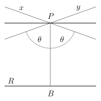
Reorganizing equation 1,
$${|PQ|}{\mathbb{H}}=k\ln\tan(\frac{\alpha}{2})$$
where $\alpha=\Pi(PQ)$ is always less than $\frac{\pi}{2}$.
${|PQ|}{\mathbb{H}}$ is positive and monotone decreasing in
The hyperbolic distance between two points
Let
$X$ be a geodesic space and$\triangle\subset X$ a geodesic triangle; that is, a set of three geodesic segments in$X$ such that any pair of segments shares precisely one endpoint. Then$\triangle$ is$\delta$ -slim if any side of$\triangle$ is contained in the$\delta$ -neighbourhood of the other two. The metric space X is$\delta$ -hyperbolic if every triangle is$\delta$ -slim, and$X$ is called hyperbolic if it is$\delta$ -hyperbolic for some$\delta\geq 0$ .
- Characterizing the analogy between hyperbolic embedding and community structure of complex networks
- Hyperbolic Embedding search result @Arxiv-sanity
- Geometric Representation Learning
- Scalable Hyperbolic Recommender Systems

- Hyperbolic Heterogeneous Information Network Embedding
- http://hyperbolicdeeplearning.com/poincare-glove/
- https://dawn.cs.stanford.edu/2018/03/19/hyperbolics/
- http://bjlkeng.github.io/posts/hyperbolic-geometry-and-poincare-embeddings/
- https://github.com/HazyResearch/hyperbolics
We have a set of distances between points,
From this we construct an inner product matrix
This matrix should be positive semidefinite with a smallest eigenvalue of zero. We can use this fact to find the appropriate radius
Point positions can then be found easily using standard kernel embedding techniques. This embedding is exact if the points lie on a hypersphere. Of course real data rarely lies precisely on a spherical manifold and so the paper also discusses details of the inexact case.
This can naturally be extended to hyperbolic embeddings where and we need to optimize the second smallest eigenvalue $$ \left<x_i, x_j\right>= -r^2\cosh(\frac{d_{ij}}{r})\ r^{\ast} = \arg\min_{r}|\lambda_2[Z(r)]|. $$
Here
| Stanford bunny texture mapped with spherical texture using spherical embedding |
|---|
 |
- Spherical and Hyperbolic Embeddings of Data
- http://simbad-fp7.eu/
- https://www.cs.york.ac.uk/cvpr/embedding/TPAMI2316836.pdf
Delaunay Graph: Given a set of vertices in the hyperbolic plane Delaunay graph is one where a pair of vertices are neighbors if their Voronoi cells intersect.
Here the Voronoi cell of
We construct a function
Edge embedding function
Here
Algorithm: Construction of
Suppose
- http://www.ae.metu.edu.tr/tuncer/ae546/prj/delaunay/
- Low Distortion Delaunay Embedding of Trees in Hyperbolic Plane
| A simple Pythagorean embedding into the vertices of a unit cube |
|---|
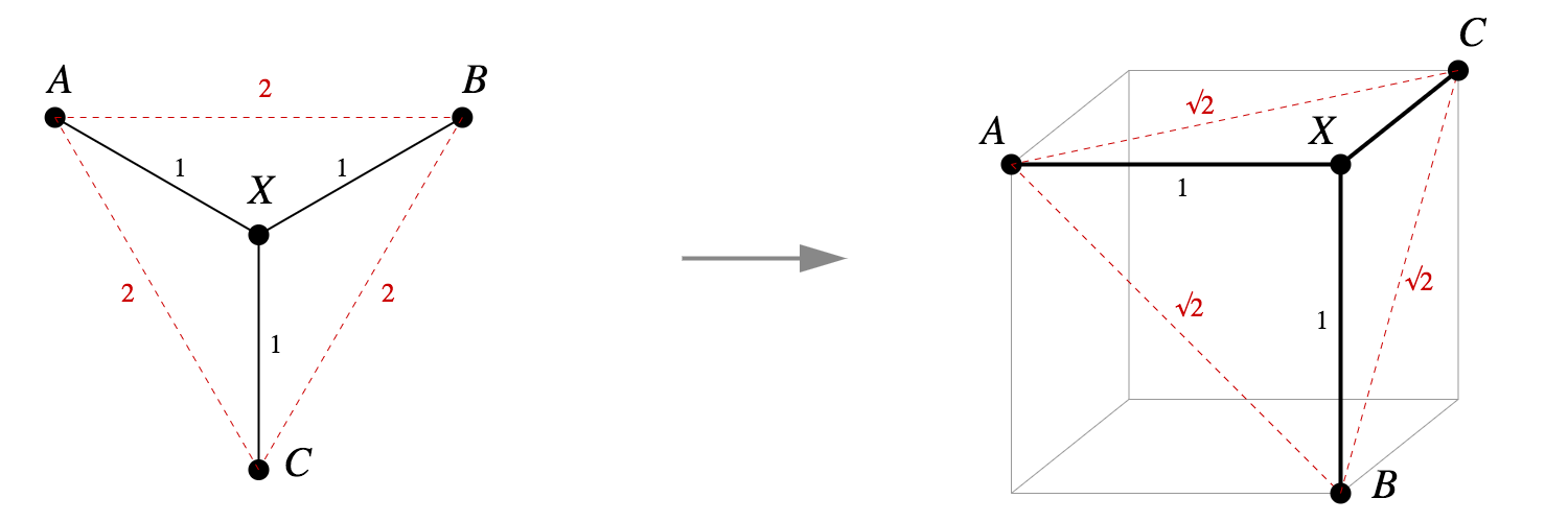 |
- A randomized embedding algorithm for trees
- Tree Preserving Embedding
- Language, trees, and geometry in neural networks
The Poincaré ball model is a model of n-dimensional hyperbolic geometry in which all points are embedded in an n-dimensional sphere (or in a circle in the 2D case which is called the Poincaré disk model). This is being presented second because it is much less intuitive but can be derived directly from the hyperboloid model.
The distance between two points
| An attempt at embedding a tree with branching factor 4 into the Euclidean plane | Embedding a hierarchical tree with branching factor two into a 2D hyperbolic plane |
|---|---|
 |
 |
- Poincaré Embeddings for Learning Hierarchical Representations
- Implementing Poincaré Embeddings
- Hyperbolic Geometry and Poincaré Embeddings
- http://hyperbolicdeeplearning.com/poincare-glove/
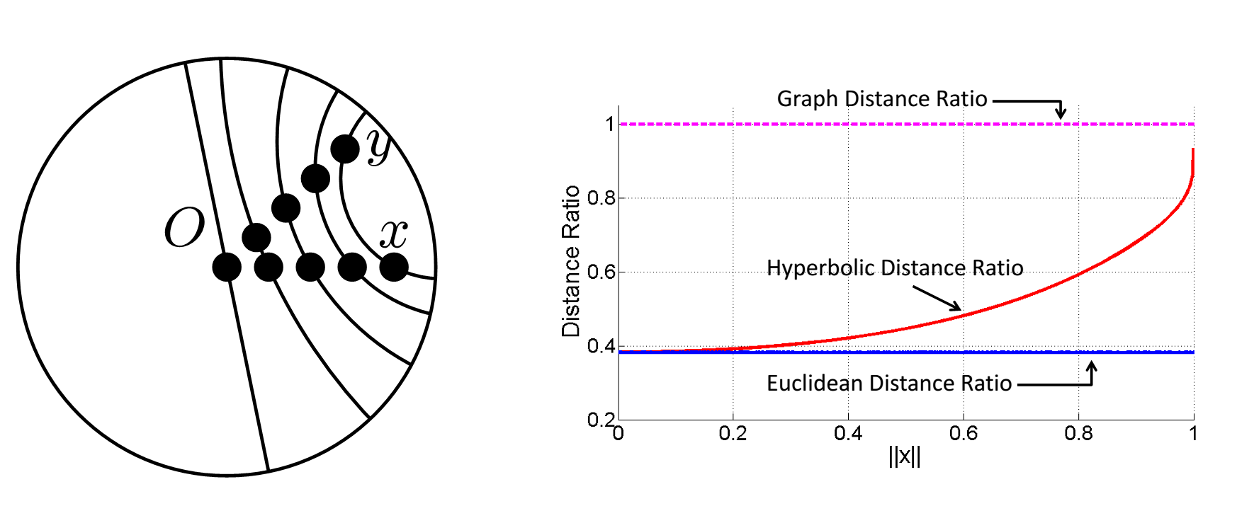
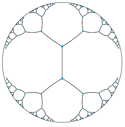
Since hyperbolic space is tree-like, it’s natural to consider embedding trees—which we can do with arbitrarily low distortion, for any number of dimensions! It is shown that how to extend this technique to arbitrary graphs, a problem with a lot of history in Euclidean space using a two-step strategy for embedding graphs into hyperbolic space:
- Embed a graph
$G = (V, E)$ into a tree$T$ . - Embed
$T$ into the Poincaré ball.
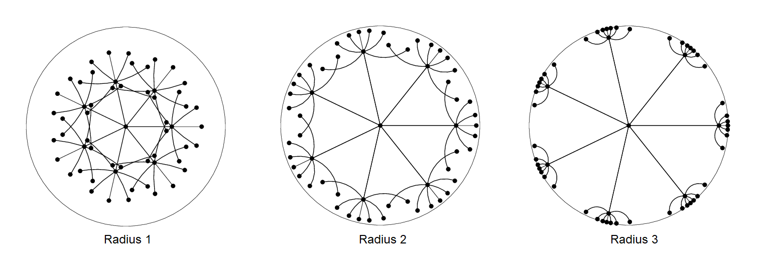
There are two factors to good embeddings: local and global. Locally, the children of each node should be spread out on the sphere around the parent. Globally, subtrees should be separated from each other; in hyperbolic space, the separation is determined by the sphere radius.
- Hyperbolic Embeddings with a Hopefully Right Amount of Hyperbole
- Hyperbolic Function Embedding: Learning Hierarchical Representation for Functions of Source Code in Hyperbolic Spaces
- Embedding Networks in Hyperbolic Spaces
- Statistics on Manifolds
- Analysis of Network Data
- Efficient embedding of complex networks to hyperbolic space via their Laplacian
- Hyperbolic geometry and real life networks
- Neural Embeddings of Graphs in Hyperbolic Space
- Metric Embedding, Hyperbolic Space, and Social Networks∗
In this website, we release hyperbolic embeddings that can be further integrated into applications related to knowledge base completion or can be supplied as features into various NLP tasks such as Question Answering.
| --- | --- |
|---|---|
 |
 |
- https://zhuanlan.zhihu.com/p/47489505
- http://blog.lcyown.cn/2018/04/30/graphencoding/
- https://blog.csdn.net/NockinOnHeavensDoor/article/details/80661180
- http://building-babylon.net/2018/04/10/graph-embeddings-in-hyperbolic-space/
- https://paperswithcode.com/task/graph-embedding
- Representation Tradeoffs for Hyperbolic Embeddings
Graph embedding, preprocessing of graph data processing, is an example of representation learning to find proper numerical representation form of graph data structure.
It maps the graph structure to numerical domain:
- Graph Embedding:深度学习推荐系统的"基本操作"
- https://github.com/thunlp/NRLpapers
- https://github.com/thunlp/GNNPapers
- http://snap.stanford.edu/proj/embeddings-www/
- https://arxiv.org/abs/1709.05584
- http://cazabetremy.fr/Teaching/EmbeddingClass.html
- https://posenhuang.github.io/
- https://jangunmp1.github.io/
- http://rischanlab.github.io/
- https://shiruipan.github.io/
- https://tksaha.github.io/
- https://fajieyuan.github.io/
- https://frostliu.github.io/
- https://papislatam2018.sched.com/
- Awesome Graph Embedding
- A Beginner's Guide to Graph Analytics and Deep Learning
- 15TH INTERNATIONAL WORKSHOP ON MINING AND LEARNING WITH GRAPHS
- Network Embedding as Matrix Factorization: Unifying DeepWalk, LINE, PTE, and node2vec
- Spatially Embedded Networks
- DOOCN-XII: Network Representation Learning
- Representation Learning on Graphs: Methods and Applications
- GEM: Graph Embedding and Mining
- Graph Exploration and Mining at Scale (GEMS) lab
- Beyond Graph Mining - Higher-Order Data Analytics for Temporal Network Data
- Scalable. Interactive. Interpretable.
- https://sites.google.com/site/mingnus/algorithms/graph-mining
DeepWalk is an approach for learning latent representations of vertices in a network, which maps the nodes in the graph into real vectors:
$$
f: \mathbb{V}\to\mathbb{R}^{d}.
$$
DeepWalk generalizes recent advancements in language modeling and unsupervised feature learning (or deep learning) from sequences of words to graphs. DeepWalk uses local information obtained from truncated random walks to learn latent representations by treating walks as the equivalent of sentences.
And if we consider the text as digraph, word2vec is an specific example of DeepWalk.
Given the word sequence
- DeepWalk
$G, w, d, \gamma, t$
- Input: graph
$G(V, E)$ ; window size$w$ ; embedding size$d$ ; walks per vertex$\gamma$ ; walk length$t$ .- Output: matrix of vertex representations
$\Phi\in\mathbb{R}^{|V|\times d}$
- Initialization: Sample
$\Phi$ from$\mathbb{U}^{|V|\times d}$ ;
- Build a binary Tree T from V;
- for
$i = 0$ to$\gamma$ do
$O = Shuffle(V )$ - for each
$v_i \in O$ do$W_{v_i}== RandomWalk(G, v_i, t)$ $SkipGram(Φ, W_{v_i}, w)$ - end for
- end for
$SkipGram(Φ, W_{v_i}, w)$
-
- for each
$v_j \in W_{v_i}$ do
-
- for each
$u_k \in W_{v_i}[j - w : j + w]$ do
- for each
-
$J(\Phi)=-\log Pr(u_k\mid \Phi(v_j))$
-
$\Phi =\Phi -\alpha\frac{\partial J}{\partial \Phi}$
-
- end for
- for each
-
- end for
Computing the partition function (normalization factor) is expensive, so instead we will factorize the
conditional probability using Hierarchical softmax.
If the path to vertex
Now,
- DeepWalk: Online Learning of Social Representations
- DeepWalk at github
- Deep Walk Project @perozzi.net
- http://www.cnblogs.com/lavi/p/4323691.html
- https://www.ijcai.org/Proceedings/16/Papers/547.pdf
node2vec is an algorithmic framework for representational learning on graphs. Given any graph, it can learn continuous feature representations for the nodes, which can then be used for various downstream machine learning tasks.
By extending the Skip-gram architecture to networks, it seeks to optimize the following objective function,
which maximizes the log-probability of observing a network neighborhood
Conditional independence and Symmetry in feature space are expected to make the optimization problem tractable.
We model the conditional likelihood of every source-neighborhood node pair as a softmax
unit parametrized by a dot product of their features:
$$
Pr(n_i\mid f(u))=\frac{\exp(f(n_i)\cdot f(u))}{\sum_{v\in V} \exp(f(v)\cdot f(u))}.
$$
The objective function simplifies to
- https://zhuanlan.zhihu.com/p/30599602
- http://snap.stanford.edu/node2vec/
- https://cs.stanford.edu/~jure/pubs/node2vec-kdd16.pdf
- https://www.kdd.org/kdd2016/papers/files/rfp0218-groverA.pdf
This is a paper about identifying nodes in graphs that play a similar role based solely on the structure of the graph, for example computing the structural identity of individuals in social networks. That’s nice and all that, but what I personally find most interesting about the paper is the meta-process by which the authors go about learning the latent distributed vectors that capture the thing they’re interested in (structural similarity in this case). Once you’ve got those vectors, you can do vector arithmetic, distance calculations, use them in classifiers and other higher-level learning tasks and so on. As word2vec places semantically similar words close together in space, so we want structurally similar nodes to be close together in space.
Struc2vec has four main steps:
- Determine the structural similarity between each vertex pair in the graph, for different neighborhood sizes.
- Construct a weighted multi-layer graph, in which each layer corresponds to a level in a hierarchy measuring structural similarity (think: ‘at this level of zoom, these things look kind of similar?).
- Use the multi-layer graph to generate context for each node based on biased random walking.
- Apply standard techniques to learn a latent representation from the context given by the sequence of nodes in the random walks.

- STRUC2VEC(图结构→向量)论文方法解读
- struc2vec: Learning Node Representations from Structural Identity
- https://arxiv.org/abs/1704.03165
- Struc2vec: learning node representations from structural identity
- metapath2vec: Scalable Representation Learning for Heterogeneous Networks
- https://ericdongyx.github.io/
- Representation Learning on Networks
- International Workshop on Deep Learning for Graphs and Structured Data Embedding
http://koaning.io/gaussian-auto-embeddings.html
M. V. Diudea, I. Gutman and L. Jantschi wrote in the preface of the book Molecular Topology: One of the principal goals of chemistry is to establish (causal) relations between the chemical and physical (experimentally observable and measurable) properties of substance and the structure of the corresponding molecules. Countless results along these lines have been obtained, and their presentation comprise significant parts of textbooks of organic, inorganic and physical chemistry, not to mention treatises on theoretical chemistry
- RDF2Vec: RDF Graph Embeddings and Their Applications
- EmbedS: Scalable and Semantic-Aware Knowledge Graph Embeddings
graph2vec is to learn data-driven distributed representations of arbitrary sized graphs in an unsupervised manner and are task agnostic.
- graph2vec: Learning Distributed Representations of Graphs
- https://allentran.github.io/graph2vec
- http://humanativaspa.it/tag/graph2vec/
- https://zhuanlan.zhihu.com/p/33732033
- Awesome graph embedding
- Graph Embedding Methods
- Graph Embedding @ deep learning pattern
- LINE: Large-scale Information Network Embedding
- Latent Network Summarization: Bridging Network Embedding and Summarization
- NodeSketch: Highly-Efficient Graph Embeddings via Recursive Sketching
- GEMS Lab
- Graph Embeddings — The Summary
- Graph Embeddings search result @ Arxiv-sanity
- Semantic Annotation for Places in LBSN through Graph Embedding
- https://ai.googleblog.com/2019/06/innovations-in-graph-representation.html
- Hierarchical Representations with Poincaré Variational Auto-Encoders
- Nonparametric Variational Auto-encoders for Hierarchical Representation Learnings
- Poincaré Embeddings for Learning Hierarchical Representations
