
In the last decade, Deep Learning approaches (e.g. Convolutional Neural Networks and Recurrent Neural Networks) allowed to achieve unprecedented performance on a broad range of problems coming from a variety of different fields (e.g. Computer Vision and Speech Recognition). Despite the results obtained, research on DL techniques has mainly focused so far on data defined on Euclidean domains (i.e. grids). Nonetheless, in a multitude of different fields, such as: Biology, Physics, Network Science, Recommender Systems and Computer Graphics; one may have to deal with data defined on non-Euclidean domains (i.e. graphs and manifolds). The adoption of Deep Learning in these particular fields has been lagging behind until very recently, primarily since the non-Euclidean nature of data makes the definition of basic operations (such as convolution) rather elusive. Geometric Deep Learning deals in this sense with the extension of Deep Learning techniques to graph/manifold structured data.
- Into the Wild: Machine Learning In Non-Euclidean Spaces
- https://jian-tang.com/teaching/graph2019
- Introducing Grakn & Knowledge Graph Convolutional Networks: Dec 4, 2018 · Paris, France
- International Workshop on Deep Learning for Graphs and Structured Data Embedding
- HYPERBOLIC DEEP LEARNING: A nascent and promising field
- https://www.minds.jhu.edu/tripods/
- https://sites.google.com/view/goergen/research
Images are stored in computer as matrix roughly. The spatial distribution of pixel on the screen project to us a colorful digitalized world.
Convolutional neural network(ConvNet or CNN) has been proved to be efficient to process and analyses the images for visual cognitive tasks.
What if we generalize these methods to graph structure which can be represented as adjacent matrix?
| Image | Graph |
|---|---|
| Convolutional Neural Network | Graph Convolution Network |
| Attention | Graph Attention |
| Gated | Gated Graph Network |
| Generative | Generative Models for Graphs |
Advanced proceedings of natural language processing(NLP) shone a light into semantic embedding as one potential approach to knowledge representation.
The text or symbol, strings in computer, is designed for natural people to communicate and understand based on the context or situation, i.e., the connections of entities and concepts are essential.
What if we generalize these methods to connected data?
- Why Deep Learning Works: A Manifold Disentanglement Perspective
- Manifold Learning of Brain MRIs by Deep Learning
- http://www.cs.cornell.edu/~kilian/index.html
- https://www.researchgate.net/profile/Taco_Cohen2
- https://github.com/tscohen
- https://zhuanlan.zhihu.com/p/34042888
Recall the recursive form of forward neural network: $$ X\to \underbrace{\sigma}{nonlinerality}\circ \underbrace{(\underbrace{W_1X}{\text{Matrix-vector multiplication}}+b_1)}_{\text{Bias translation}}=H_1\to \cdots \sigma(WH+b)=y. $$
It consists of matrix-vector multiplication, vector addition, nonlinear transformation and function composition.
The hyperbolic hyperplane centered at

The hyperbolic softmax probabilities are given by
- Hyperbolic Neural Networks
- http://hyperbolicdeeplearning.com/papers/
- http://hyperbolicdeeplearning.com/
- http://hyperbolicdeeplearning.com/hyperbolic-neural-networks/
- https://github.com/ferrine/hyrnn
- https://cla2019.github.io/
- https://github.com/alex-tifrea
- http://shichuan.org/
- https://www.cgal.org/project.html
- Learning Mixed-Curvature Representations in Product Spaces

The Möbius addition of
The Möbius scalar multiplication of
Likewise, this operation satisfies a few properties:
- Associativity:
$$r \otimes(s \otimes x) = (r \otimes s) \otimes x$$ - additions: $$ n \otimes x=x \oplus \cdots \oplus x(n \text { times })$$
- Scalar distributivity:
$$(r+s) \otimes x=(r \otimes x) \oplus(s \otimes x)$$ - Scaling property:
$$r \otimes x /|r \otimes x|=x /|x|.$$
The geodesic between two points
A manifold
Then, if you take a vector
- Moving
$x$ to the tangent space at$0$ of the Poincaré ball using$\log_0$ , - Multiplying this vector by
$r$ , since$\log_0(x)$ is now in the vector space$T_x\mathbb{D}^n=\mathbb{R}^n$ , - Projecting it back on the manifold using the exp map at
$0$ .

We propose to define matrix-vector multiplications in the Poincaré ball in a similar manner:
- Matrix associativity:
$M\otimes (N\otimes x)\ = (MN)\otimes x$ - Compatibility with scalar multiplication:
$M\otimes (r\otimes x)\ = (rM)\otimes x = r\otimes(M\otimes x)$ - Directions are preserved:
$M\otimes x/\parallel M\otimes x\parallel = Mx/\parallel Mx\parallel$ for$Mx\neq 0$ - Rotations are preserved:
$M\otimes x= Mx$ for$M\in\mathcal{O}_n(\mathbb{R})$
In order to generalize multinomial logistic regression (MLR, also called softmax regression), we proceed in 3 steps:
We first reformulate softmax probabilities with a distance to a margin hyperplane Second, we define hyperbolic hyperplanes Finally, by finding the closed-form formula of the distance between a point and a hyperbolic hyperplane, we derive the final formula.
Similarly as for the hyperbolic GRU, we show that when the Poincaré ball in continuously flattened to Euclidean space (sending its radius to infinity), hyperbolic softmax converges to Euclidean softmax.
- http://hyperbolicdeeplearning.com/hyperbolic-neural-networks/
- https://github.com/dalab/hyperbolic_nn
A natural adaptation of RNN using our formulas yields:
$$ \begin{array}{l}{r_{t}=\sigma \log_{0}\left(\left(\left(W^{r} \otimes h_{t-1}\right) \oplus\left(U^{r} \otimes x_{t}\right)\right) \oplus b^{r}\right)} \ { z_{t}=\sigma \log_{0}\left(\left(\left(W^{z} \otimes h_{t-1}\right) \oplus\left(U^{z} \otimes x_{t}\right)\right) \oplus b^{z}\right)} \ {\left.\tilde{h}{t}=\varphi^{\otimes}\left(\left(\left(W \operatorname{diag}\left(r{t}\right)\right] \otimes h_{t-1}\right) \oplus\left(U \otimes x_{t}\right)\right) \oplus b\right)} \ {h_{t}=h_{t-1} \oplus\left(\operatorname{diag}\left(z_{t}\right) \otimes\left(\left(-h_{t-1}\right) \oplus \widetilde{h_{t}}\right)\right)}\end{array} $$
- Hyperbolic Attention Networks
- https://openreview.net/forum?id=rJxHsjRqFQ
- https://sites.google.com/site/eccvgdl/
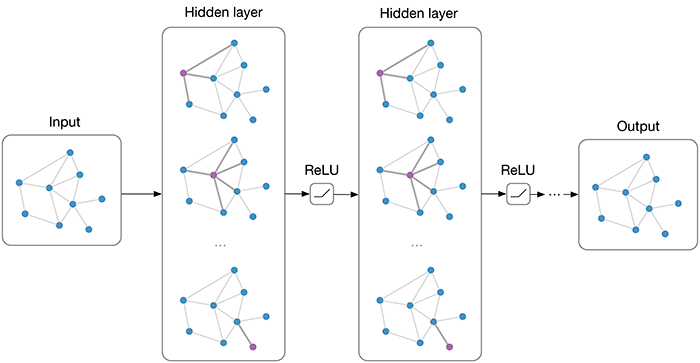
If images is regarded as a matrix in computer and text as a chain( or sequence), their representation contain all the spatial and semantic information of the entity.
Graph can be represented as adjacency matrix as shown in Graph Algorithm. However, the adjacency matrix only describe the connections between the nodes.
The feature of the nodes does not appear. The node itself really matters.
For example, the chemical bonds can be represented as adjacency matrix while the atoms in molecule really determine the properties of the molecule.
A simple and direct way is to concatenate the feature matrix adjacency matrix
And what is the output? How can deep learning apply to them? And how can we extend the tree-based algorithms such as decision tree into graph-based algorithms?
For these models, the goal is then to learn a function of signals/features on a graph
$G=(V,E)$ which takes as input:
- A feature description
$x_i$ for every node$i$ ; summarized in a$N\times D$ feature matrix${X}$ ($N$ : number of nodes,$D$ : number of input features);- A representative description of the graph structure in matrix form; typically in the form of an adjacency matrix
${A}$ (or some function thereof)
and produces a node-level output
$Z$ (an$N\times F$ feature matrix, where$F$ is the number of output features per node). Graph-level outputs can be modeled by introducing some form of pooling operation (see, e.g. Duvenaud et al., NIPS 2015).
Every neural network layer can then be written as a non-linear function
$$
{H}{i+1} = \sigma \circ ({H}{i}, A)
$$
with ${H}0 = {X}{in}$ and
For example, we can consider a simple form of a layer-wise propagation rule
$$
{H}{i+1} = \sigma \circ ({H}{i}, A)=\sigma \circ(A {H}{i} {W}{i})
$$
where
-
But first, let us address two limitations of this simple model: multiplication with
$A$ means that, for every node, we sum up all the feature vectors of all neighboring nodes but not the node itself (unless there are self-loops in the graph). We can "fix" this by enforcing self-loops in the graph: we simply add the identity matrix$I$ to$A$ . -
The second major limitation is that
$A$ is typically not normalized and therefore the multiplication with$A$ will completely change the scale of the feature vectors (we can understand that by looking at the eigenvalues of$A$ ).Normalizing${A}$ such that all rows sum to one, i.e.$D^{-1}A$ , where$D$ is the diagonal node degree matrix, gets rid of this problem.
In fact, the propagation rule introduced in Kipf & Welling (ICLR 2017) is given by:
$$
{H}{i+1} = \sigma \circ ({H}{i}, A)=\sigma \circ(\hat{D}^{-\frac{1}{2}} \hat{A} \hat{D}^{-\frac{1}{2}} {H}{i} {W}{i}),
$$
with
Like other neural network, GCN is also composite of linear and nonlinear mapping. In details,
-
$\hat{D}^{-\frac{1}{2}} \hat{A} \hat{D}^{-\frac{1}{2}}$ is to normalize the graph structure; - the next step is to multiply node properties and weights;
- Add nonlinearities by activation function
$\sigma$ .
See more at experoinc.com or https://tkipf.github.io/.

Neural nets do well on vectors and tensors; data types like images (which have structure embedded in them via pixel proximity – they have fixed size and spatiality); and sequences such as text and time series (which display structure in one direction, forward in time).
Graphs have an arbitrary structure: they are collections of things without a location in space, or with an arbitrary location. They have no proper beginning and no end, and two nodes connected to each other are not necessarily “close”.
GCN can be regarded as the counterpart of CNN for graphs so that the optimization techniques such as normalization, attention mechanism and even the adversarial version can be extended to the graph structure.
- A Beginner's Guide to Graph Analytics and Deep Learning
- Node Classification by Graph Convolutional Network
- https://benevolent.ai/publications
- https://missinglink.ai/guides/convolutional-neural-networks/graph-convolutional-networks/
- Lecture 11: Learning on Non-Euclidean Domains: Prof. Alex Bronstein
- FastGCN: Fast Learning with Graph Convolutional Networks via Importance Sampling
Compositional layers of convolutional neural network can be expressed as
$$ \hat{H}{i} = P\oplus H{i-1} \ \tilde{H_i} = C_i\otimes(\hat{H}_{t}) \ Z_i = \mathrm{N}\cdot \tilde{H_i} \ H_i = Pooling\cdot (\sigma\circ Z_i) $$
where
Xavier Bresson gave a talk on New Deep Learning Techniques FEBRUARY 5-9, 2018. We would ideally like our graph convolutional layer to have:
- Computational and storage efficiency (requiring no more than
$O(E+V)$ time and memory); - Fixed number of parameters (independent of input graph size);
- Localisation (acting on a local neighbourhood of a node);
- Ability to specify arbitrary importances to different neighbours;
- Applicability to inductive problems (arbitrary, unseen graph structures).
| CNN | GCN | --- |
|---|---|---|
| padding | ? | ? |
| convolution | ? | Information of neighbors |
| pooling | ? | Invariance |
-
Spectral graph theoryallows to redefine convolution in the context of graphs with Fourier analysis. - Graph downsampling
$\iff$ graph coarsening$\iff$ graph partitioning: Decompose${G}$ into smaller meaningful clusters. - Structured pooling: Arrangement of the node indexing such that adjacent nodes are hierarchically merged at the next coarser level.
Laplacian operator is represented as a positive semi-definite
| Laplacian | Representation |
|---|---|
| Unnormalized Laplacian | |
| Normalized Laplacian | |
| Random walk Laplacian | |
|
|
|
Eigendecomposition of graph Laplacian:
where
Convolution of two vectors
where the last equation is because the matrix multiplication is associative and
The spectral definition of a convolution-like operation on a non-Euclidean domain allows to parametrize the action of a filter as
where
To mimick the construction of a regular CNN, we construct a spectral convolutional layer accepting an m-dimensional vertex field
Graph Convolution: Recursive Computation with Shared Parameters:
- Represent each node based on its neighborhood
- Recursively compute the state of each node by propagating previous states using relation specific transformations
- Backpropagation through Structure
We would like to impose spatial localization onto the weights
Every graph convolutional layer starts off with a shared node-wise feature transformation (in order to achieve a higher-level representation), specified by a weight matrix
In general, to satisfy the localization property, we will define a graph convolutional operator as an aggregation of features across neighborhoods;
defining
Parametrize the smooth spectral filter function
- SplineNets: Continuous Neural Decision Graphs
- Spatial CNN
- a-comprehensive-survey-on-graph-neural-networks
Represent smooth spectral functions with polynomials of Laplacian eigenvalues $$w_{\alpha}(\lambda)={\sum}{j=0}^r{\alpha}{j} {\lambda}^j$$
where
Convolutional layer: Apply spectral filter to feature signal
Such graph convolutional layers are GPU friendly.
Graph convolution network always deal with unstructured data sets where the graph has different size. What is more, the graph is dynamic, and we need to apply to new nodes without model retraining.
Graph convolution with (non-orthogonal) monomial basis
Kipf and Welling proposed the ChebNet (arXiv:1609.02907) to approximate the filter using Chebyshev polynomial.
Application of the filter with the scaled Laplacian:
$$w_{\alpha}(\tilde{\mathbf{\Delta}})f= {\sum}{j=0}^r{\alpha}{j} T_j({\tilde{\mathbf{\Delta}}}) f={\sum}{j=0}^r{\alpha}{j}X^{(j)}$$
with
- Graph Convolutional Neural Network (Part I)
- The Promise of Deep Learning on Graphs
- https://www.ntu.edu.sg/home/xbresson/
- https://github.com/xbresson
Use Chebychev polynomials of degree
Further constrain


In the previous post, the convolution of the graph Laplacian is defined in its graph Fourier space as outlined in the paper of Bruna et. al. (arXiv:1312.6203). However, the eigenmodes of the graph Laplacian are not ideal because it makes the bases to be graph-dependent. A lot of works were done in order to solve this problem, with the help of various special functions to express the filter functions. Examples include Chebyshev polynomials and Cayley transform.
Graph Convolution Networks (GCNs) generalize the operation of convolution from traditional data (images or grids) to graph data.
The key is to learn a function f to generate
a node
Defining filters as polynomials applied over the eigenvalues of the graph Laplacian, it is possible
indeed to avoid any eigen-decomposition and realize convolution by means of efficient sparse routines
The main idea behind CayleyNet is to achieve some sort of spectral zoom property by means of Cayley transform:
$$
C(\lambda) = \frac{\lambda - i}{\lambda + i}
$$
Instead of Chebyshev polynomials, it approximates the filter as:
$$
g(\lambda) = c_0 + \sum_{j=1}^{r}[c_jC^{j}(h\lambda) + c_j^{\ast} C^{j^{\ast}}(h\lambda)]
$$
where ChebNet.
- CayleyNets: Graph Convolutional Neural Networks with Complex Rational Spectral Filters
- CayleyNets at IEEE
MotifNet is aimed to address the directed graph convolution.

- MotifNet: a motif-based Graph Convolutional Network for directed graphs
- Neural Motifs: Scene Graph Parsing with Global Context (CVPR 2018)
- GCN Part II @datawarrior
- http://mirlab.org/conference_papers/International_Conference/ICASSP%202018/pdfs/0006852.pdf
Minimal inner structures:
- Invariant by vertex re-indexing (no graph matching is required)
- Locality (only neighbors are considered) Weight sharing (convolutional operations)
- Independence w.r.t. graph size
- Higher-order Graph Convolutional Networks
- A Higher-Order Graph Convolutional Layer
- MixHop: Higher-Order Graph Convolutional Architectures via Sparsified Neighborhood Mixing
- https://zhuanlan.zhihu.com/p/62300527
- https://zhuanlan.zhihu.com/p/64498484
- https://zhuanlan.zhihu.com/p/28170197
- Wavelets on Graphs via Spectral Graph Theory
- Spectral Networks and Locally Connected Networks on Graphs
Graph convolutional layer then computes a set of new node features, $(\vec{h}{1},\cdots, \vec{h}{n})$ , based on the input features as well as the graph structure.
Most prior work defines the kernels
In Graph Attention Networks the kernels
We inject the graph structure by only allowing node

- Generative Models for Graphs by David White & Richard Wilson
- Generative Graph Convolutional Network for Growing Graphs
- BAYESIAN GRAPH CONVOLUTIONAL NEURAL NETWORKS USING NON-PARAMETRIC GRAPH LEARNING
- https://rlgm.github.io/
- https://www.octavian.ai/
- https://github.com/huawei-noah/BGCN
- https://github.com/thunlp/GNNPapers
- graph convolution network 有什么比较好的应用task? - 知乎
- Use of graph network in machine learning
- Node Classification by Graph Convolutional Network
- Semi-Supervised Classification with Graph Convolutional Networks
GCN for RecSys
PinSAGE Node’s neighborhood defines a computation graph. The key idea is to generate node embeddings based on local neighborhoods. Nodes aggregate information from their neighbors using neural networks.
- Graph Neural Networks for Social Recommendation
- 图神经网+推荐
- Graph Convolutional Neural Networks for Web-Scale Recommender Systems
- Graph Convolutional Networks for Recommender Systems
GCN for Bio & Chem
- DeepChem is a Python library democratizing deep learning for science.
- Chemi-Net: A molecular graph convolutional network for accurate drug property prediction
- Chainer Chemistry: A Library for Deep Learning in Biology and Chemistry
- Release Chainer Chemistry: A library for Deep Learning in Biology and Chemistry
- Modeling Polypharmacy Side Effects with Graph Convolutional Networks
- http://www.grakn.ai/?ref=Welcome.AI
- AlphaFold: Using AI for scientific discovery
- A graph-convolutional neural network model for the prediction of chemical reactivity
- Convolutional Networks on Graphs for Learning Molecular Fingerprints
- A graph-convolutional neural network model for the prediction of chemical reactivity
GCN for NLP
- https://www.akbc.ws/2019/
- http://www.akbc.ws/2017/slides/ivan-titov-slides.pdf
- https://github.com/icoxfog417/graph-convolution-nlp
- https://nlp.stanford.edu/pubs/zhang2018graph.pdf
- https://cs.stanford.edu/people/jure/
- https://github.com/alibaba/euler
- https://ieeexplore.ieee.org/document/8439897
- Higher-order organization of complex networks
- Geometric Matrix Completion with Recurrent Multi-Graph Neural Networks
- http://snap.stanford.edu/proj/embeddings-www/
- http://ryanrossi.com/
- http://www.ipam.ucla.edu/programs/workshops/geometry-and-learning-from-data-tutorials/
- https://zhuanlan.zhihu.com/p/51990489
- https://www.cs.toronto.edu/~yujiali/
- https://olki.loria.fr/
- https://qdata.github.io/deep2Read/
- https://www.ee.iitb.ac.in/~eestudentrg/
- 2019 Graph Signal Processing Workshop
- Machine Learning for 3D Data
- Geometric Deep Learning @qdata
- https://qdata.github.io/deep2Read//aReadingsIndexByCategory/#2Graphs
- The Power of Graphs in Machine Learning and Sequential Decision-Making
- http://geometricdeeplearning.com/
- Artificial Intelligence and Augmented Intelligence for Automated Investigations for Scientific Discovery
- Learning the Structure of Graph Neural Networks Mathias Niepert, NEC Labs Europe July 09, 2019
- https://sites.google.com/site/rdftestxyz/home
- Lecture 11: Learning on Non-Euclidean Domains
- What Can Neural Networks Reason About?
- Deep Geometric Matrix Completion by Federico Monti
- https://pytorch-geometric.readthedocs.io/en/latest/
- https://deeplearning-cmu-10707.github.io/
- 3D Machine Learning
- https://nthu-datalab.github.io/ml/index.html
- http://www.pmp-book.org/
- https://github.com/rubenwiersma/cgthesis
- http://deeplearning.lipingyang.org/
- http://vgl.ict.usc.edu/Research/GeometricDeepLearning/
- https://idl.cs.washington.edu/
- Python for NLP
- Deep Learning on Graphs: A Survey
- Graph-based Neural Networks
- Geometric Deep Learning
- Deep Chem
- GRAM: Graph-based Attention Model for Healthcare Representation Learning
- https://zhuanlan.zhihu.com/p/49258190
- https://www.zhihu.com/question/54504471
- http://sungsoo.github.io/2018/02/01/geometric-deep-learning.html
- https://rusty1s.github.io/pytorch_geometric/build/html/notes/introduction.html
- .mp4 illustration
- Deep Graph Library (DGL)
- https://github.com/alibaba/euler
- https://github.com/alibaba/euler/wiki/%E8%AE%BA%E6%96%87%E5%88%97%E8%A1%A8
- https://www.groundai.com/project/graph-convolutional-networks-for-text-classification/
- https://datawarrior.wordpress.com/2018/08/08/graph-convolutional-neural-network-part-i/
- https://datawarrior.wordpress.com/2018/08/12/graph-convolutional-neural-network-part-ii/
- http://www.cs.nuim.ie/~gunes/files/Baydin-MSR-Slides-20160201.pdf
- http://colah.github.io/posts/2015-09-NN-Types-FP/
- https://www.zhihu.com/question/305395488/answer/554847680