Kar Ng 2021
- 1 SUMMARY
- 2 R PACKAGES
- 3 INTRODUCTION
- 3 EXPERIMENTAL DESIGN SUMMARY
- 4 DATA PREPARATION
- 5 DATA CLEANING AND MANIPULATION
- 6 EXPLORATORY DATA ANALYSIS (EDA)
- 7 STATISTICAL ANALYSIS
- 8 CONCLUSION
- 9 LEGALITY
- 10 REFERENCE
Reading time: 14 minutes
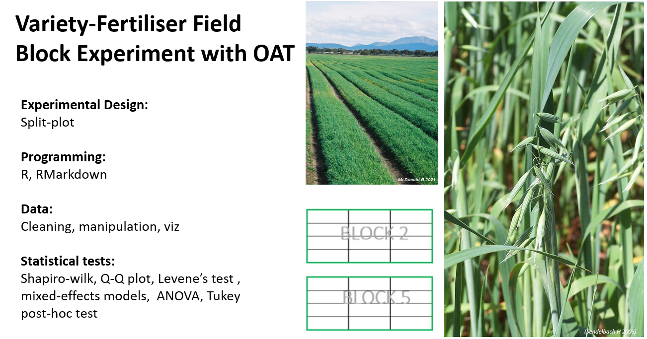
The main purpose of this project is to demonstrate my experimentation and analytically skills using R programming language. This project is about analyzing an oat dataset collected from a Split-plot research system. It is a common but more advanced research method for a factorial agricultural experiment that works on multiple independent variables. The experiment was carried out in a field. The experimentation field was spitted into block, plot, and subplot.
There are 3 independent variables in the dataset with various levels. They are 6 blocks, 3 oat varieties, and 4 nutrient levels. Responding variable was plant yield in kilogram per hectare. Exploratory data analysis (EDA) was carried out to explore general trends of the dataset, then followed by statistical analyses. This project uses a mixed-effect model to analyse significant differences among oat varieties, nutrient levels (manurial nitrogen) and their interactions. Statistical assumptions were tests using Q-Q plot, Shapiro-Wilk test, and Levene’s test. Results from the test shown normality among residuals and variances among treatment groups were the same. ANOVA and Tukey were selected as the omnibus and post-hoc test.
Results reveal that there is no significant yield difference among oat varieties. However, there is significant yield difference between nutrient levels. There is no significant interaction effect between oat varieties and nutrient levels. If a decision has to be made, my top 3 best combinations selected from the dataset will be the three varieties, Marvellous, Golden rain, and Victory, with 50 kilogram per hectare of manurial nitrogen application. It is the second highest nutrient level from the experiment. I am not picking the highest nutrient level that had the best yield because the yield though was higher but is not significantly higher than my top 3 recommendations. These recommendations may also more beneficial for farm economics and surrounding environment.
Highlights

R packages loaded in this project include tidyverse packages (ggplot2, dplyr, tidyr, readr, purrr, tibble, stringr, and forcats), skimr, lubridate, kableEtra, agridat, MASS, DescTools, DescTools, lme4, qqplotr, lsmeans, and multcomp.
library(tidyverse)
library(skimr)
library(lubridate)
library(kableExtra)
library(agridat)
library(MASS)
library(DescTools)
library(lme4)
library(lmerTest)
library(qqplotr)
library(lsmeans)
library(multcomp)
library(pbkrtest)
library(multcompView) # To use CLD methodsThis personal project uses a public dataset from an oat field experiment, the data was available for download from a R package called MASS. The objective of this project is to demonstrate how I successfully analyse the data using statistical methods to find out the optimum nutrient levels on different variety of oats, with incorporation of the effects of blocks and plots.
The experiment was carried out in a field with a famous agricultural experimentation system called split plot. This method splits the entire allocated field into different blocks and further subdividing into smaller plots and even smaller subplots. In the dataset, there are 3 oat varieties and 4 levels of manurial treatment (nutrient level).
The experiment was,
- laid out in 6 blocks as 6 replicates,
- each block has 3 main plots splitted for the 3 type of oat varieties,
- and there are 4 subplots in each plot for 4 levels of nutrient treatments.
A sketch to visualise the arrangement of blocks. The arrangement of each block is often subjected to the direction of gradient of identified heterogeneous environment.

I am expecting all treatments were randomised within plot. It is a usual way to minimize the impact of heterogeneous environmental conditions for more accurate results. For example, if the left corner has more soil moisture than the right corner, then having a randomised plots would avoid particular treatment be assigned to the heterogeneous corner and generating unfairn data.

Fundamentals of split-plot and RCBD are similar. RCBD (Randomisation Complete Block Design) stops when the split achieves plots, whereas split plot further splits the plots into subplots. They are widely-used experimental designs in agriculture research to minimise heterogeneous field conditions. These conditions can be sporadic soil water availability, inherent nutrient contents, soil chemistry, or other environmental conditions in the research field. These effects on the crops can be ranged from small to large. Usually, when a heterogeneous condition is identified, blocks will be arranged in a gradient against the identified area. It is to ensure the heterogeneous area has all treatments in it. Therefore, it can reduce biases against particular treatments and reduce overall experimental errors because all treatments have now equal chance receiving the heterogeneous soil conditions.
In general, one can assume which variable in a split-plot experiment is the most important variable for the researchers by looking at where the variable is being plotted. Usually, the variable that assigned to the subplot is the variable that interest the researchers the most, which is “nutrient level on oat” in this case. The second interest of this split plot experiment is the variable assigned to the plot, which is the “varieties” of oat in this case.
- Crop: Oat
- Experimental Design: Split-Plot
- Experimental unit: Subplot
- Independent variables: Varieties, Nutrient levels
- Levels of independent variable: 3 Varieties, 4 nutrient levels
- Number of treatment group: 12 (3 varieties x 4 nutrient levels)
- Number of replication: 6
- Dependent variable: Plant yield
To fully examine the yield of oats due to varieties and nutrient levels in a split plots. I will need to statistically analyse and compare the effects of varieties, nutrient levels, their interaction, and the effects of plots and subplots.
Following code import the data and the table indicates successful import of the dataset.
data("oats")
oats
## B V N Y
## 1 I Victory 0.0cwt 111
## 2 I Victory 0.2cwt 130
## 3 I Victory 0.4cwt 157
## 4 I Victory 0.6cwt 174
## 5 I Golden.rain 0.0cwt 117
## 6 I Golden.rain 0.2cwt 114
## 7 I Golden.rain 0.4cwt 161
## 8 I Golden.rain 0.6cwt 141
## 9 I Marvellous 0.0cwt 105
## 10 I Marvellous 0.2cwt 140
## 11 I Marvellous 0.4cwt 118
## 12 I Marvellous 0.6cwt 156
## 13 II Victory 0.0cwt 61
## 14 II Victory 0.2cwt 91
## 15 II Victory 0.4cwt 97
## 16 II Victory 0.6cwt 100
## 17 II Golden.rain 0.0cwt 70
## 18 II Golden.rain 0.2cwt 108
## 19 II Golden.rain 0.4cwt 126
## 20 II Golden.rain 0.6cwt 149
## 21 II Marvellous 0.0cwt 96
## 22 II Marvellous 0.2cwt 124
## 23 II Marvellous 0.4cwt 121
## 24 II Marvellous 0.6cwt 144
## 25 III Victory 0.0cwt 68
## 26 III Victory 0.2cwt 64
## 27 III Victory 0.4cwt 112
## 28 III Victory 0.6cwt 86
## 29 III Golden.rain 0.0cwt 60
## 30 III Golden.rain 0.2cwt 102
## 31 III Golden.rain 0.4cwt 89
## 32 III Golden.rain 0.6cwt 96
## 33 III Marvellous 0.0cwt 89
## 34 III Marvellous 0.2cwt 129
## 35 III Marvellous 0.4cwt 132
## 36 III Marvellous 0.6cwt 124
## 37 IV Victory 0.0cwt 74
## 38 IV Victory 0.2cwt 89
## 39 IV Victory 0.4cwt 81
## 40 IV Victory 0.6cwt 122
## 41 IV Golden.rain 0.0cwt 64
## 42 IV Golden.rain 0.2cwt 103
## 43 IV Golden.rain 0.4cwt 132
## 44 IV Golden.rain 0.6cwt 133
## 45 IV Marvellous 0.0cwt 70
## 46 IV Marvellous 0.2cwt 89
## 47 IV Marvellous 0.4cwt 104
## 48 IV Marvellous 0.6cwt 117
## 49 V Victory 0.0cwt 62
## 50 V Victory 0.2cwt 90
## 51 V Victory 0.4cwt 100
## 52 V Victory 0.6cwt 116
## 53 V Golden.rain 0.0cwt 80
## 54 V Golden.rain 0.2cwt 82
## 55 V Golden.rain 0.4cwt 94
## 56 V Golden.rain 0.6cwt 126
## 57 V Marvellous 0.0cwt 63
## 58 V Marvellous 0.2cwt 70
## 59 V Marvellous 0.4cwt 109
## 60 V Marvellous 0.6cwt 99
## 61 VI Victory 0.0cwt 53
## 62 VI Victory 0.2cwt 74
## 63 VI Victory 0.4cwt 118
## 64 VI Victory 0.6cwt 113
## 65 VI Golden.rain 0.0cwt 89
## 66 VI Golden.rain 0.2cwt 82
## 67 VI Golden.rain 0.4cwt 86
## 68 VI Golden.rain 0.6cwt 104
## 69 VI Marvellous 0.0cwt 97
## 70 VI Marvellous 0.2cwt 99
## 71 VI Marvellous 0.4cwt 119
## 72 VI Marvellous 0.6cwt 121
Following table describes what is each column of the dataset comprised of.
Variables <- c("B", "V", "N", "Y")
Description <- c("Blocks, levels I, II, III, IV, V, VI",
                 "Variesties, 3 levels",
                 "Nitrogen (manurial) treatment, levels 0.0cwt, 0.2cwt, 0.4cwt, 0.6cwt, showing the application in unit of cwt/acre",
                 "Yields in 1/4lbs per sub-plot, each of area 1/80 acre.")

data.frame(Variables, Description) %>%
  kbl() %>%
kable_styling(bootstrap_options = c("bordered", "stripped", "hover"))| Variables | Description |
|---|---|
| B | Blocks, levels I, II, III, IV, V, VI |
| V | Variesties, 3 levels |
| N | Nitrogen (manurial) treatment, levels 0.0cwt, 0.2cwt, 0.4cwt, 0.6cwt, showing the application in unit of cwt/acre |
| Y | Yields in 1/4lbs per sub-plot, each of area 1/80 acre. |
The dataset has 74 rows of observations and 4 columns of variables. There are 3 variables, B, V, and N, categorised as factor, and the Y is categorised as numerical data.
skim_without_charts(oats)| Name | oats |
| Number of rows | 72 |
| Number of columns | 4 |
| \_\_\_\_\_\_\_\_\_\_\_\_\_\_\_\_\_\_\_\_\_\_\_ | |
| Column type frequency: | |
| factor | 3 |
| numeric | 1 |
| \_\_\_\_\_\_\_\_\_\_\_\_\_\_\_\_\_\_\_\_\_\_\_\_ | |
| Group variables | None |
Variable type: factor
| skim\_variable | n\_missing | complete\_rate | ordered | n\_unique | top\_counts |
|---|---|---|---|---|---|
| B | 0 | 1 | FALSE | 6 | I: 12, II: 12, III: 12, IV: 12 |
| V | 0 | 1 | FALSE | 3 | Gol: 24, Mar: 24, Vic: 24 |
| N | 0 | 1 | FALSE | 4 | 0.0: 18, 0.2: 18, 0.4: 18, 0.6: 18 |
Variable type: numeric
| skim\_variable | n\_missing | complete\_rate | mean | sd | p0 | p25 | p50 | p75 | p100 |
|---|---|---|---|---|---|---|---|---|---|
| Y | 0 | 1 | 103.97 | 27.06 | 53 | 86 | 102.5 | 121.25 | 174 |
The data set is complete and having no missing data. It can be examined through the results of the columns n_missing and complete_rate. The two columns associate with missing value in each column of the dataset. All variables (B, V, N and Y) have 0 in the n_missing, and 1 in the complete_rate throughout their columns.
Following is the summary of the dataset.
summary(oats)## B V N Y
## I :12 Golden.rain:24 0.0cwt:18 Min. : 53.0
## II :12 Marvellous :24 0.2cwt:18 1st Qu.: 86.0
## III:12 Victory :24 0.4cwt:18 Median :102.5
## IV :12 0.6cwt:18 Mean :104.0
## V :12 3rd Qu.:121.2
## VI :12 Max. :174.0
- There are 6 blocks.
- There are 3 oat varieties.
- There are 4 nutrient levels.
- The range of the overall yield can be ranged from minimum of 53 lbs/acre to maximum of 174 lbs/acre, with mean of 104 lbs/acre and median of 102.5 lbs/acre.
The dataset is obviously has been cleaned by the up-loader of the dataset. The dataset has been transformed to a long format already, all variables have been assigned to their desired types, having no missing values and unnecessary spaces to trim.
Rename variables
However, variable names of B, V, N, and Y can be changed to a more complete, simple, intuitive terms such as block, variety, nutrient, and yield, to make them more sensible and understandable for readers who are not familiar with the dataset.
Following codes complete the changes (click the right button), and the table reveals the outcome of the codes.
oat <- oats %>%             # note: I change the name of oats to oat, to preserve original dataset.
  rename("block" = "B",
         "variety" = "V",
         "nutrient" = "N",
         "yield" = "Y")

oat
## block variety nutrient yield
## 1 I Victory 0.0cwt 111
## 2 I Victory 0.2cwt 130
## 3 I Victory 0.4cwt 157
## 4 I Victory 0.6cwt 174
## 5 I Golden.rain 0.0cwt 117
## 6 I Golden.rain 0.2cwt 114
## 7 I Golden.rain 0.4cwt 161
## 8 I Golden.rain 0.6cwt 141
## 9 I Marvellous 0.0cwt 105
## 10 I Marvellous 0.2cwt 140
## 11 I Marvellous 0.4cwt 118
## 12 I Marvellous 0.6cwt 156
## 13 II Victory 0.0cwt 61
## 14 II Victory 0.2cwt 91
## 15 II Victory 0.4cwt 97
## 16 II Victory 0.6cwt 100
## 17 II Golden.rain 0.0cwt 70
## 18 II Golden.rain 0.2cwt 108
## 19 II Golden.rain 0.4cwt 126
## 20 II Golden.rain 0.6cwt 149
## 21 II Marvellous 0.0cwt 96
## 22 II Marvellous 0.2cwt 124
## 23 II Marvellous 0.4cwt 121
## 24 II Marvellous 0.6cwt 144
## 25 III Victory 0.0cwt 68
## 26 III Victory 0.2cwt 64
## 27 III Victory 0.4cwt 112
## 28 III Victory 0.6cwt 86
## 29 III Golden.rain 0.0cwt 60
## 30 III Golden.rain 0.2cwt 102
## 31 III Golden.rain 0.4cwt 89
## 32 III Golden.rain 0.6cwt 96
## 33 III Marvellous 0.0cwt 89
## 34 III Marvellous 0.2cwt 129
## 35 III Marvellous 0.4cwt 132
## 36 III Marvellous 0.6cwt 124
## 37 IV Victory 0.0cwt 74
## 38 IV Victory 0.2cwt 89
## 39 IV Victory 0.4cwt 81
## 40 IV Victory 0.6cwt 122
## 41 IV Golden.rain 0.0cwt 64
## 42 IV Golden.rain 0.2cwt 103
## 43 IV Golden.rain 0.4cwt 132
## 44 IV Golden.rain 0.6cwt 133
## 45 IV Marvellous 0.0cwt 70
## 46 IV Marvellous 0.2cwt 89
## 47 IV Marvellous 0.4cwt 104
## 48 IV Marvellous 0.6cwt 117
## 49 V Victory 0.0cwt 62
## 50 V Victory 0.2cwt 90
## 51 V Victory 0.4cwt 100
## 52 V Victory 0.6cwt 116
## 53 V Golden.rain 0.0cwt 80
## 54 V Golden.rain 0.2cwt 82
## 55 V Golden.rain 0.4cwt 94
## 56 V Golden.rain 0.6cwt 126
## 57 V Marvellous 0.0cwt 63
## 58 V Marvellous 0.2cwt 70
## 59 V Marvellous 0.4cwt 109
## 60 V Marvellous 0.6cwt 99
## 61 VI Victory 0.0cwt 53
## 62 VI Victory 0.2cwt 74
## 63 VI Victory 0.4cwt 118
## 64 VI Victory 0.6cwt 113
## 65 VI Golden.rain 0.0cwt 89
## 66 VI Golden.rain 0.2cwt 82
## 67 VI Golden.rain 0.4cwt 86
## 68 VI Golden.rain 0.6cwt 104
## 69 VI Marvellous 0.0cwt 97
## 70 VI Marvellous 0.2cwt 99
## 71 VI Marvellous 0.4cwt 119
## 72 VI Marvellous 0.6cwt 121
The changes have been successfully completed.
Convert the units of nutrient and yield
The unit of nutrient is cwt/arce, and the unit of yield is lbs/acre. Personally, I am more comfortable with the unit kg/ha or ton/ha. The conversion is optional but I will carry out the conversion in this section, with:
- 1 cwt = 50.8023 kg
- 1 acre = 0.404686 ha
- 1 lbs = 0.453592 kg
Following codes complete the conversion (click right button) and the table reveals the outcome of the codes.
oat2 <- oat %>%
  mutate(nutrient = str_remove(nutrient, "cwt"),
         nutrient = as.numeric(nutrient),
         nutrient = round(nutrient*50.8023/0.404686),
         nutrient = as.factor(nutrient),
         yield = round(yield * 0.453592/0.404686))

oat2
## block variety nutrient yield
## 1 I Victory 0 124
## 2 I Victory 25 146
## 3 I Victory 50 176
## 4 I Victory 75 195
## 5 I Golden.rain 0 131
## 6 I Golden.rain 25 128
## 7 I Golden.rain 50 180
## 8 I Golden.rain 75 158
## 9 I Marvellous 0 118
## 10 I Marvellous 25 157
## 11 I Marvellous 50 132
## 12 I Marvellous 75 175
## 13 II Victory 0 68
## 14 II Victory 25 102
## 15 II Victory 50 109
## 16 II Victory 75 112
## 17 II Golden.rain 0 78
## 18 II Golden.rain 25 121
## 19 II Golden.rain 50 141
## 20 II Golden.rain 75 167
## 21 II Marvellous 0 108
## 22 II Marvellous 25 139
## 23 II Marvellous 50 136
## 24 II Marvellous 75 161
## 25 III Victory 0 76
## 26 III Victory 25 72
## 27 III Victory 50 126
## 28 III Victory 75 96
## 29 III Golden.rain 0 67
## 30 III Golden.rain 25 114
## 31 III Golden.rain 50 100
## 32 III Golden.rain 75 108
## 33 III Marvellous 0 100
## 34 III Marvellous 25 145
## 35 III Marvellous 50 148
## 36 III Marvellous 75 139
## 37 IV Victory 0 83
## 38 IV Victory 25 100
## 39 IV Victory 50 91
## 40 IV Victory 75 137
## 41 IV Golden.rain 0 72
## 42 IV Golden.rain 25 115
## 43 IV Golden.rain 50 148
## 44 IV Golden.rain 75 149
## 45 IV Marvellous 0 78
## 46 IV Marvellous 25 100
## 47 IV Marvellous 50 117
## 48 IV Marvellous 75 131
## 49 V Victory 0 69
## 50 V Victory 25 101
## 51 V Victory 50 112
## 52 V Victory 75 130
## 53 V Golden.rain 0 90
## 54 V Golden.rain 25 92
## 55 V Golden.rain 50 105
## 56 V Golden.rain 75 141
## 57 V Marvellous 0 71
## 58 V Marvellous 25 78
## 59 V Marvellous 50 122
## 60 V Marvellous 75 111
## 61 VI Victory 0 59
## 62 VI Victory 25 83
## 63 VI Victory 50 132
## 64 VI Victory 75 127
## 65 VI Golden.rain 0 100
## 66 VI Golden.rain 25 92
## 67 VI Golden.rain 50 96
## 68 VI Golden.rain 75 117
## 69 VI Marvellous 0 109
## 70 VI Marvellous 25 111
## 71 VI Marvellous 50 133
## 72 VI Marvellous 75 136
Now, the units of nutrient and yield have been converted into kg/ha.
After cleaning, the very first step is always visualising the data because it is the time one can have a chance to have a general understanding of the dataset, what are the obvious trends, how data points are spread out, and how each levels of variables are visually different from each other.
My EDA will explore:
- 6.1 Yield vs Variety
- 6.2 Yield vs Nutrient Level
- 6.3 Yield vs Blocks
- 6.4 Yield vs Variety + Nutrient Level
- 6.5 Yield vs Variety + Nutrient level + Blocks
There is no obvious yield difference among oat varieties. If a comparison is needed to be made, the Marvellous has the highest average yield, followed by Golden rain, then Victory. However, the differences are not much.
# set up df

df6.1 <- oat2 %>%
  dplyr::select(variety, yield) %>%                         # MASS package making select of dplyr error, having dplyr:: solve the issue.
  group_by(variety) %>%
  mutate(count = n(),
         xlab = as.factor(paste0(variety, "\n", "(n = ", count, ")")))


ggplot(df6.1, aes(x = reorder(xlab, -yield), y = yield, fill = variety, colour = variety)) +
  geom_boxplot(alpha = 0.1, outlier.shape = NA) +
  stat_boxplot(geom = "errorbar") +
  geom_jitter(width = 0.2) +
  stat_summary(fun.y = mean, geom = "point", size = 7, shape = 4, stroke = 2) +
  labs(x = "Oat Variety",
       y = "Yield, kg/ha",
       title = "Figure 1. There is no obvious yield different between Oat Varietes",
       subtitle = " 'x' in the boxplot represents mean.") +
  theme_bw() +
  theme(legend.position = "none",
        axis.title.x = element_text(margin = margin(10, 0, 0, 0)),
        plot.title = element_text(face = "bold", vjust = 1))
The yield of oat increased with increasing nutrient content. A positive relationship is observed. However, a subtle insight should be noted which is the rate of yield increment from 50 kg/ha of nitrogen to 75 kg/ha is not as much as from 0 kg/ha to 25 kg/ha and from 25 kg/ha to 50 kg/ha.
# set up df

df6.2 <- oat2 %>%
  dplyr::select(nutrient, yield) %>%                         # MASS package making select of dplyr error, having dplyr:: solve the issue.
  group_by(nutrient) %>%
  mutate(count = n(),
         xlab = as.factor(paste0(nutrient, "\n", "(n = ", count, ")")))


ggplot(df6.2, aes(x = reorder(xlab, yield), y = yield, fill = nutrient, colour = nutrient)) +
  geom_boxplot(alpha = 0.1, outlier.shape = NA) +
  stat_boxplot(geom = "errorbar") +
  geom_jitter(width = 0.2) +
  stat_summary(fun.y = mean, geom = "point", size = 7, shape = 4, stroke = 2) +
  labs(x = "Nutrient levels, kg/ha",
       y = "Yield, kg/ha",
       title = "Figure 2. Oat yields increased with increasing Nutrient Content",
       subtitle = " 'x' in the boxplot represents mean.") +
  theme_bw() +
  theme(legend.position = "none",
        axis.title.x = element_text(margin = margin(10, 0, 0, 0)),
        plot.title = element_text(face = "bold", vjust = 1))
An important question for farmer is that whether the smaller increment of yield at the 2 highest nutrient levels outweigh the cost of the additional nutrient added.
This section is important to observe yields among blocks. In a most basic experimental design, blocks are often treated as replicates and each replicates should be free from environmental noises, meaning the results between each block should be similar.
However, perhaps Block 1 has been identified to have a condition that favors plant growth. This would be a reason why split-plot is selected compared to a CRD (completely randomised design) to account for the heterogeneous condition.
# set up df

df6.3 <- oat2 %>%
  dplyr::select(block, yield) %>%                         # MASS package making select of dplyr error, having dplyr:: solve the issue.
  group_by(block) %>%
  mutate(count = n(),
         xlab = as.factor(paste0(block, "\n", "(n = ", count, ")")))


ggplot(df6.3, aes(x = reorder(xlab, -yield), y = yield, fill = block, colour = block)) +
  geom_boxplot(alpha = 0.1, outlier.shape = NA) +
  stat_boxplot(geom = "errorbar") +
  geom_jitter(width = 0.2) +
  stat_summary(fun.y = mean, geom = "point", size = 7, shape = 4, stroke = 2) +
  labs(x = "Block",
       y = "Yield, kg/ha",
       title = "Figure 3. Yield in Block I has the Highest Yield than Other Blocks",
       subtitle = " 'x' in the boxplot represents mean.") +
  theme_bw() +
  theme(legend.position = "none",
        axis.title.x = element_text(margin = margin(10, 0, 0, 0)),
        plot.title = element_text(face = "bold", vjust = 1))
Again, the type of statistical analysis from the split-block design allows one to account for the errors (noises) between blocks. Additionally, difference among plots will also be accounted in the statistical analysis section, which further increases the accuracy of the result.
Following graph summarises the effects of oat varieties and nutrient contents in the soil on yield.
# set up df

df6.4 <- oat2 %>%
  dplyr::select(variety, nutrient, yield)                 # MASS package making select of dplyr error, having dplyr:: solve the issue.


ggplot(df6.4, aes(x = variety, y = yield, fill = nutrient)) +
  geom_boxplot(alpha = 0.8, outlier.shape = NA) +
  stat_boxplot(geom = "errorbar") +
  geom_point(position = position_jitterdodge(), width = 0.1, size = 2, shape = 21, aes(fill = nutrient)) +
  stat_summary(fun.y = mean, geom = "point", size = 5, shape = 4, position = position_jitterdodge(0), colour = "blue", stroke = 1.5) +
  labs(x = "Block",
       y = "Yield, kg/ha",
       title = "Figure 4. The Effect of Variety + Nutrient on Oat Yield.",
       subtitle = " 'x' in the boxplot represents mean.",
       fill = "Nutrient level, kg/ha: ") +
  theme_bw() +
  theme(legend.position = "bottom",
        axis.title.x = element_text(margin = margin(10, 0, 0, 0)),
        plot.title = element_text(face = "bold", vjust = 1)) +
scale_fill_manual(values = c("yellow", "green1", "green2", "green4")) 
- Victory variety always has the lowest yield across all nutrient levels compared to other varieties.
- There are consistent outliers observed throughout individual nutrient treatment of Victory.
- The outliers can be due to the effect of block. 6 data points of each boxplot are planted in 6 different blocks. It is highly likely that there is an effect of block. If it is true, a statistical analysis that taking block into account is important for more accurate results.
Following figure 5 has too many variables and making it less effective in story telling. I hope my addition of light to dark green to highlight different nutrient levels will aid you a little.
Insights:
- The outliers observed in the victory of afore figure 4 could be planted in block I because yields in block 1 is visually higher than other blocks.
- 75 kg/ha of nutrient level (N) has always the highest yield but not most of the times, sometime 50 kg/ha of N nutrient is higher.
- In all blocks, there is not much visually difference in yield between oat varieties.
# set up df

df6.5 <- oat2 %>%
  group_by(block, variety) %>%
  mutate(count = n(),
         xlab = as.factor(paste0(variety, "\n", "(n = ", count, ")")))

ggplot(df6.5, aes(x = variety, y = yield, fill = nutrient)) +
  geom_bar(stat = "identity", position = "dodge", colour = "black") +
  facet_wrap(~block) +
  labs(x = "Oat Variety",
       y = "Yield, kg/ha",
       fill = "Nutrient level, kg/ha: ",
       title = "Figure 5. Oat Yield of Different Treatments in Different Blocks") +
  theme_bw() +
  theme(legend.position = "bottom",
        axis.title.x = element_text(margin = margin(10, 0, 0, 0)),
        plot.title = element_text(face = "bold", vjust = 1)) +
scale_fill_manual(values = c("yellow", "green1", "green2", "green4")) 
The statistical analysis for split plot design requires a model that takes both fixed and random effects into account. Fixed effect include the variety, nutrient, and the interaction of these two variables. Random effects include the blocks and the plots. Assuming some residuals may be the effect of blocks and plots due to their inherent differences despite the effects might be insignificant and the researchers have done their best in choosing a research field. The model will still incorporate and consider errors due to these random effects.
Prior to all processes, my usual first step is assumptions checking, it includes the testing of the normality of residuals, and data variances among all possible combination of treatments. This steps are important to decide what omnibus and post-hoc tests.
Building the model
model <- lmer(yield ~ variety + nutrient + variety:nutrient + (1|block) + (1|block:variety),
              data = oat2)
summary(model)
## Linear mixed model fit by REML. t-tests use Satterthwaite's method [
## lmerModLmerTest]
## Formula: yield ~ variety + nutrient + variety:nutrient + (1 | block) +
## (1 | block:variety)
## Data: oat2
##
## REML criterion at convergence: 542.8
##
## Scaled residuals:
## Min 1Q Median 3Q Max
## -1.81365 -0.55118 0.02205 0.64379 1.57713
##
## Random effects:
## Groups Name Variance Std.Dev.
## block:variety (Intercept) 133.3 11.54
## block (Intercept) 268.9 16.40
## Residual 223.1 14.94
## Number of obs: 72, groups: block:variety, 18; block, 6
##
## Fixed effects:
## Estimate Std. Error df t value Pr(>|t|)
## (Intercept) 89.6667 10.2086 16.1263 8.783 1.52e-07 ***
## varietyMarvellous 7.6667 10.8993 30.2658 0.703 0.4872
## varietyVictory -9.8333 10.8993 30.2658 -0.902 0.3741
## nutrient25 20.6667 8.6237 45.0000 2.397 0.0208 *
## nutrient50 38.6667 8.6237 45.0000 4.484 5.02e-05 ***
## nutrient75 50.3333 8.6237 45.0000 5.837 5.45e-07 ***
## varietyMarvellous:nutrient25 3.6667 12.1957 45.0000 0.301 0.7651
## varietyVictory:nutrient25 0.1667 12.1957 45.0000 0.014 0.9892
## varietyMarvellous:nutrient50 -4.6667 12.1957 45.0000 -0.383 0.7038
## varietyVictory:nutrient50 5.8333 12.1957 45.0000 0.478 0.6347
## varietyMarvellous:nutrient75 -5.5000 12.1957 45.0000 -0.451 0.6542
## varietyVictory:nutrient75 2.6667 12.1957 45.0000 0.219 0.8279
## ---
## Signif. codes: 0 '***' 0.001 '**' 0.01 '*' 0.05 '.' 0.1 ' ' 1
##
## Correlation of Fixed Effects:
## (Intr) vrtyMr vrtyVc ntrn25 ntrn50 ntrn75 vrM:25 vrV:25 vrM:50
## vartyMrvlls -0.534
## varityVctry -0.534 0.500
## nutrient25 -0.422 0.396 0.396
## nutrient50 -0.422 0.396 0.396 0.500
## nutrient75 -0.422 0.396 0.396 0.500 0.500
## vrtyMrvl:25 0.299 -0.559 -0.280 -0.707 -0.354 -0.354
## vrtyVctr:25 0.299 -0.280 -0.559 -0.707 -0.354 -0.354 0.500
## vrtyMrvl:50 0.299 -0.559 -0.280 -0.354 -0.707 -0.354 0.500 0.250
## vrtyVctr:50 0.299 -0.280 -0.559 -0.354 -0.707 -0.354 0.250 0.500 0.500
## vrtyMrvl:75 0.299 -0.559 -0.280 -0.354 -0.354 -0.707 0.500 0.250 0.500
## vrtyVctr:75 0.299 -0.280 -0.559 -0.354 -0.354 -0.707 0.250 0.500 0.250
## vrV:50 vrM:75
## vartyMrvlls
## varityVctry
## nutrient25
## nutrient50
## nutrient75
## vrtyMrvl:25
## vrtyVctr:25
## vrtyMrvl:50
## vrtyVctr:50
## vrtyMrvl:75 0.250
## vrtyVctr:75 0.500 0.500
Normality of residuals
- Residues generated from the mixed effect model of the dataset are
normally distributed, supported by,
- The following Q-Q plot that most of the points are lying close to the line and are mostly within the 95% confidence shaded area around the line.
oat2$resid <- resid(model)
ggplot(oat2, aes(sample = resid)) +
  stat_qq_band() +
  stat_qq_line() +
  stat_qq_point() +
  labs(title = "Q-Q plot",
       subtitle = "model = lmer(yield ~ variety + nutrient + variety:nutrient + (1|block) + (1|block:variety),
              data = oat2)") +
  theme(plot.title = element_text(face = "bold"))
* The
normality is also supported by Shapiro-Wilk test that test on the
residuals of the model and having a p-value of 0.2811, which is higher
than 0.05, and fail to reject the null hypothesis that the residuals are
normally distributed.
* The
normality is also supported by Shapiro-Wilk test that test on the
residuals of the model and having a p-value of 0.2811, which is higher
than 0.05, and fail to reject the null hypothesis that the residuals are
normally distributed.
shapiro.test(resid(model))##
## Shapiro-Wilk normality test
##
## data: resid(model)
## W = 0.97928, p-value = 0.2811
Spread of variances
Applying Levene’s test to test the spread of variances among levels within two of the fixed effect variables - “variety” and “nutrient”. Levene’s tests show that variances among the treatment groups of variety are equal to each other, with P-value higher than 0.05. The variances among the treatment groups of nutrient level also equal to each other (P-value > 0.05).
LeveneTest(oat2$yield ~ oat2$variety)## Levene's Test for Homogeneity of Variance (center = median)
## Df F value Pr(>F)
## group 2 0.4424 0.6443
## 69
LeveneTest(oat2$yield ~ oat2$nutrient)## Levene's Test for Homogeneity of Variance (center = median)
## Df F value Pr(>F)
## group 3 0.0501 0.9851
## 68
Base on the results of assumption tests in the previous section, anova is selected as the omnibus test to find out are there differences between groups.
print(anova(model))## Type III Analysis of Variance Table with Satterthwaite's method
## Sum Sq Mean Sq NumDF DenDF F value Pr(>F)
## variety 668.4 334.2 2 10 1.4979 0.2698
## nutrient 25195.2 8398.4 3 45 37.6436 2.502e-12 ***
## variety:nutrient 418.0 69.7 6 45 0.3122 0.9273
## ---
## Signif. codes: 0 '***' 0.001 '**' 0.01 '*' 0.05 '.' 0.1 ' ' 1
Computed ANOVA table shows that the F-value of nutrient treatment is very high which indicating that the variances between groups is significantly higher than variances within group and resulting a highly significant P-value of way lesser than 0.05. There are no significant difference between oat varieties, as well as interaction between oat varieties and nutrient levels.
Since there is significant result from the omnibus test, post-hoc test is allowed to be proceeded. The column “.group” shows a summary of the statistical results with letters. Letters that overlapped each other are not significant different or otherwise (P = 0.05).
Post-hoc for Nutrient only
ls_n <- lsmeans(model, ~nutrient)
lscld_n <- cld(ls_n, Letters = LETTERS, reversed = T)
lscld_n
## nutrient lsmean SE df lower.CL upper.CL .group
## 75 138.3 8.04 6.8 119.2 157 A
## 50 128.0 8.04 6.8 108.9 147 A
## 25 110.9 8.04 6.8 91.8 130 B
## 0 88.9 8.04 6.8 69.8 108 C
##
## Results are averaged over the levels of: variety
## Degrees-of-freedom method: kenward-roger
## Confidence level used: 0.95
## P value adjustment: tukey method for comparing a family of 4 estimates
## significance level used: alpha = 0.05
## NOTE: Compact letter displays can be misleading
## because they show NON-findings rather than findings.
## Consider using 'pairs()', 'pwpp()', or 'pwpm()' instead.
A 95% confidence interval plot is also a very helpful visualisation.
ggplot(lscld_n, aes(x = nutrient, y = lsmean, colour = nutrient)) +
  geom_errorbar(aes(ymin = lower.CL, ymax = upper.CL), size = 2) +
  geom_point(size = 6) +
  geom_text(aes(label = .group), vjust = -6, stroke = 1.5) +
  scale_y_continuous(lim = c(60, 180), breaks = seq(60, 180, 20)) +
  theme_classic() +
  theme(legend.position = "none",
        plot.title = element_text(face = "bold")) +
  labs(title = "CI Plot: Nutrient levels",
       x = "Nutrient level, kg/ha",
       y = "Plant yield, kg/ha")
Insights:
- Nutrients levels at 50 kg/ha and 75 kg/ha have significant higher plant yield than 0 kg/ha and 25 kg/ha.
- However, two of the 50 kg/ha and 75 kg/ha nutrients level are not significantly different from each other.
- This plot does not separate out the data from 3 varieties of oats.
A final overall post-hoc test will be computed to obverse overall differences.
Post-hoc for interaction between Nutrient and variety
Following shows the statistical results between the treatment groups of variety and nutrient. Letters that overlap each other indicating not significant different (P = 0.05).
ls_vn <- lsmeans(model, ~ variety * nutrient)
lscld_vn <- cld(ls_vn, Letters = LETTERS, reversed = T)
lscld_vn
## variety nutrient lsmean SE df lower.CL upper.CL .group
## Marvellous 75 142.2 10.2 16.1 120.5 164 A
## Golden.rain 75 140.0 10.2 16.1 118.4 162 A
## Victory 75 132.8 10.2 16.1 111.2 154 A C
## Marvellous 50 131.3 10.2 16.1 109.7 153 AB
## Golden.rain 50 128.3 10.2 16.1 106.7 150 ABCD
## Victory 50 124.3 10.2 16.1 102.7 146 ABCDE
## Marvellous 25 121.7 10.2 16.1 100.0 143 ABCDE
## Golden.rain 25 110.3 10.2 16.1 88.7 132 ABCDEF
## Victory 25 100.7 10.2 16.1 79.0 122 B DEF
## Marvellous 0 97.3 10.2 16.1 75.7 119 CDEF
## Golden.rain 0 89.7 10.2 16.1 68.0 111 EF
## Victory 0 79.8 10.2 16.1 58.2 101 F
##
## Degrees-of-freedom method: kenward-roger
## Confidence level used: 0.95
## P value adjustment: tukey method for comparing a family of 12 estimates
## significance level used: alpha = 0.05
## NOTE: Compact letter displays can be misleading
## because they show NON-findings rather than findings.
## Consider using 'pairs()', 'pwpp()', or 'pwpm()' instead.
Insights:
- Resulted nutrient levels are ordered in a top-down absolute way that the higher the nutrient level in the soil, the better the plant growth.
- All 3 oat varieties with 75 kg/ha of nutrient (N) had the highest growth.
- Marvellous is the oat variety that always had the highest yield in each nutrient level.
- Victory oat variety always had the lowest yield in each nutrient level.
Visualisualing the above result using the lsmean will be:
ggplot(lscld_vn, aes(x = nutrient, y = lsmean, colour = variety)) +
  geom_path(aes(group = variety), size = 1.5) +
  geom_point(size = 4) +
  theme_classic() +
  theme(legend.position = "none") +
  labs(title = "Interaction between Nutrient Levels and Variety",
       x = "Nutrient level, kg/ha",
       y = "Plant yield (average), kg/ha") +
  geom_text(data = lscld_vn %>% filter(nutrient == "75"),
            aes(label = variety),
            hjust = -0.2)
Base on the data from this dataset, result shows that there is no significant yield difference among Marvellous, Golden rain and Victory, with P-value of higher than 0.05. However, there is significant yield difference between nutrient levels applied in the experiment (P-value < 0.05). It implies that as long as any higher rate of given nutrient level in the experiment is added, any oat variety that used in the experiment can outcompete another variety used in the experiment, though the result might be insignificant.
It should be noted that although the highest nutrient level applied in the experiment (75 kg/ha) has a higher yield than the second highest nutrient level (50 kg/ha), the difference was not significant. The suitability of adopting the highest nutrient level in this experiment should rely on the farmer’s context, economical-feasibility, and local environmental concerns. On the other aspect, there is no significant interaction effect between oat varieties and nutrient levels applied in the experiment. Base on the variety and nutrient levels applied in the experiment, there was no evidence from the statistical result showing that one oat variety may response to the nutrient significantly than another (P-value > 0.05).
If a decision has to be made to choose the best combination of oat variety and nutrient level base on the result of this project, my own top 3 best combinations are the three varieties, Marvellous, Golden rain, and Victory, with 50 kg per ha of manurial nitrogen application. Marvellous will be my most preferred oat variety, then followed by Golden rain, and lastly the victory oat variety. I am avoiding the maximum yield with the highest rate of nitrogen application as the result of yield gained was proven not significantly (P-value > 0.05) higher from my top 3 recommendations, I am also aiming for a better farm economics and environmental outcome.
Thank you for reading!
This is a personal project created and designed for skill demonstration and non-commercial use only. All photos in this project, such as those that applied as the thumbnail are just for demonstration only, they are not related to the dataset, the location where the data were collected, and the results of this analysis.
McDonald G 2021, Raised beds – design, layout, construction and renovation, view 10 July 2021, https://www.agric.wa.gov.au/waterlogging/raised-beds-%E2%80%93-design-layout-construction-and-renovation
Sendelbach 2005, Avena sativa L (oat), viewed 05 July 2021, https://en.wikipedia.org/wiki/Oat#/media/File:Avena_sativa_L.jpg
smartcopying n.d., Quick Guide to Creative Commons, viewed 04 July 2021, https://smartcopying.edu.au/quick-guide-to-creative-commons/
Venables, W. N. and Ripley, B. D. (2002) Modern Applied Statistics with S. Fourth edition. Springer.
Wright 2021, Package ‘agridat’, CRAN, viewed 04 July 2021, http://kwstat.github.io/agridat/
Yates, F. (1935) Complex experiments, Journal of the Royal Statistical Society Suppl. 2, 181–247.
Yates, F. (1970) Experimental design: Selected papers of Frank Yates, C.B.E, F.R.S. London: Griffin.