-
Notifications
You must be signed in to change notification settings - Fork 2
/
5.4-visualizing-what-convnets-learn.py
591 lines (404 loc) · 24.1 KB
/
5.4-visualizing-what-convnets-learn.py
1
2
3
4
5
6
7
8
9
10
11
12
13
14
15
16
17
18
19
20
21
22
23
24
25
26
27
28
29
30
31
32
33
34
35
36
37
38
39
40
41
42
43
44
45
46
47
48
49
50
51
52
53
54
55
56
57
58
59
60
61
62
63
64
65
66
67
68
69
70
71
72
73
74
75
76
77
78
79
80
81
82
83
84
85
86
87
88
89
90
91
92
93
94
95
96
97
98
99
100
101
102
103
104
105
106
107
108
109
110
111
112
113
114
115
116
117
118
119
120
121
122
123
124
125
126
127
128
129
130
131
132
133
134
135
136
137
138
139
140
141
142
143
144
145
146
147
148
149
150
151
152
153
154
155
156
157
158
159
160
161
162
163
164
165
166
167
168
169
170
171
172
173
174
175
176
177
178
179
180
181
182
183
184
185
186
187
188
189
190
191
192
193
194
195
196
197
198
199
200
201
202
203
204
205
206
207
208
209
210
211
212
213
214
215
216
217
218
219
220
221
222
223
224
225
226
227
228
229
230
231
232
233
234
235
236
237
238
239
240
241
242
243
244
245
246
247
248
249
250
251
252
253
254
255
256
257
258
259
260
261
262
263
264
265
266
267
268
269
270
271
272
273
274
275
276
277
278
279
280
281
282
283
284
285
286
287
288
289
290
291
292
293
294
295
296
297
298
299
300
301
302
303
304
305
306
307
308
309
310
311
312
313
314
315
316
317
318
319
320
321
322
323
324
325
326
327
328
329
330
331
332
333
334
335
336
337
338
339
340
341
342
343
344
345
346
347
348
349
350
351
352
353
354
355
356
357
358
359
360
361
362
363
364
365
366
367
368
369
370
371
372
373
374
375
376
377
378
379
380
381
382
383
384
385
386
387
388
389
390
391
392
393
394
395
396
397
398
399
400
401
402
403
404
405
406
407
408
409
410
411
412
413
414
415
416
417
418
419
420
421
422
423
424
425
426
427
428
429
430
431
432
433
434
435
436
437
438
439
440
441
442
443
444
445
446
447
448
449
450
451
452
453
454
455
456
457
458
459
460
461
462
463
464
465
466
467
468
469
470
471
472
473
474
475
476
477
478
479
480
481
482
483
484
485
486
487
488
489
490
491
492
493
494
495
496
497
498
499
500
501
502
503
504
505
506
507
508
509
510
511
512
513
514
515
516
517
518
519
520
521
522
523
524
525
526
527
528
529
530
531
532
533
534
535
536
537
538
539
540
541
542
543
544
545
546
547
548
549
550
551
552
553
554
555
556
557
558
559
560
561
562
563
564
565
566
567
568
569
570
571
572
573
574
575
576
577
578
579
580
581
582
583
584
585
586
587
588
589
590
591
#!/usr/bin/env python
# coding: utf-8
# In[1]:
import keras
keras.__version__
# # Visualizing what convnets learn
#
# This notebook contains the code sample found in Chapter 5, Section 4 of [Deep Learning with Python](https://www.manning.com/books/deep-learning-with-python?a_aid=keras&a_bid=76564dff). Note that the original text features far more content, in particular further explanations and figures: in this notebook, you will only find source code and related comments.
#
# ----
#
# It is often said that deep learning models are "black boxes", learning representations that are difficult to extract and present in a
# human-readable form. While this is partially true for certain types of deep learning models, it is definitely not true for convnets. The
# representations learned by convnets are highly amenable to visualization, in large part because they are _representations of visual
# concepts_. Since 2013, a wide array of techniques have been developed for visualizing and interpreting these representations. We won't
# survey all of them, but we will cover three of the most accessible and useful ones:
#
# * Visualizing intermediate convnet outputs ("intermediate activations"). This is useful to understand how successive convnet layers
# transform their input, and to get a first idea of the meaning of individual convnet filters.
# * Visualizing convnets filters. This is useful to understand precisely what visual pattern or concept each filter in a convnet is receptive
# to.
# * Visualizing heatmaps of class activation in an image. This is useful to understand which part of an image where identified as belonging
# to a given class, and thus allows to localize objects in images.
#
# For the first method -- activation visualization -- we will use the small convnet that we trained from scratch on the cat vs. dog
# classification problem two sections ago. For the next two methods, we will use the VGG16 model that we introduced in the previous section.
# ## Visualizing intermediate activations
#
# Visualizing intermediate activations consists in displaying the feature maps that are output by various convolution and pooling layers in a
# network, given a certain input (the output of a layer is often called its "activation", the output of the activation function). This gives
# a view into how an input is decomposed unto the different filters learned by the network. These feature maps we want to visualize have 3
# dimensions: width, height, and depth (channels). Each channel encodes relatively independent features, so the proper way to visualize these
# feature maps is by independently plotting the contents of every channel, as a 2D image.
# Let's start by loading the model that we saved in section 5.2:
# In[2]:
from keras.models import load_model
model = load_model('cats_and_dogs_small_2.h5')
model.summary() # As a reminder.
# This will be the input image we will use -- a picture of a cat, not part of images that the network was trained on:
# In[3]:
img_path = '/Users/fchollet/Downloads/cats_and_dogs_small/test/cats/cat.1700.jpg'
# We preprocess the image into a 4D tensor
from keras.preprocessing import image
import numpy as np
img = image.load_img(img_path, target_size=(150, 150))
img_tensor = image.img_to_array(img)
img_tensor = np.expand_dims(img_tensor, axis=0)
# Remember that the model was trained on inputs
# that were preprocessed in the following way:
img_tensor /= 255.
# Its shape is (1, 150, 150, 3)
print(img_tensor.shape)
# Let's display our picture:
# In[4]:
import matplotlib.pyplot as plt
plt.imshow(img_tensor[0])
plt.show()
# In order to extract the feature maps we want to look at, we will create a Keras model that takes batches of images as input, and outputs
# the activations of all convolution and pooling layers. To do this, we will use the Keras class `Model`. A `Model` is instantiated using two
# arguments: an input tensor (or list of input tensors), and an output tensor (or list of output tensors). The resulting class is a Keras
# model, just like the `Sequential` models that you are familiar with, mapping the specified inputs to the specified outputs. What sets the
# `Model` class apart is that it allows for models with multiple outputs, unlike `Sequential`. For more information about the `Model` class, see
# Chapter 7, Section 1.
# In[5]:
from keras import models
# Extracts the outputs of the top 8 layers:
layer_outputs = [layer.output for layer in model.layers[:8]]
# Creates a model that will return these outputs, given the model input:
activation_model = models.Model(inputs=model.input, outputs=layer_outputs)
# When fed an image input, this model returns the values of the layer activations in the original model. This is the first time you encounter
# a multi-output model in this book: until now the models you have seen only had exactly one input and one output. In the general case, a
# model could have any number of inputs and outputs. This one has one input and 8 outputs, one output per layer activation.
# In[6]:
# This will return a list of 5 Numpy arrays:
# one array per layer activation
activations = activation_model.predict(img_tensor)
# For instance, this is the activation of the first convolution layer for our cat image input:
# In[7]:
first_layer_activation = activations[0]
print(first_layer_activation.shape)
# It's a 148x148 feature map with 32 channels. Let's try visualizing the 3rd channel:
# In[8]:
import matplotlib.pyplot as plt
plt.matshow(first_layer_activation[0, :, :, 3], cmap='viridis')
plt.show()
# This channel appears to encode a diagonal edge detector. Let's try the 30th channel -- but note that your own channels may vary, since the
# specific filters learned by convolution layers are not deterministic.
# In[9]:
plt.matshow(first_layer_activation[0, :, :, 30], cmap='viridis')
plt.show()
# This one looks like a "bright green dot" detector, useful to encode cat eyes. At this point, let's go and plot a complete visualization of
# all the activations in the network. We'll extract and plot every channel in each of our 8 activation maps, and we will stack the results in
# one big image tensor, with channels stacked side by side.
# In[10]:
import keras
# These are the names of the layers, so can have them as part of our plot
layer_names = []
for layer in model.layers[:8]:
layer_names.append(layer.name)
images_per_row = 16
# Now let's display our feature maps
for layer_name, layer_activation in zip(layer_names, activations):
# This is the number of features in the feature map
n_features = layer_activation.shape[-1]
# The feature map has shape (1, size, size, n_features)
size = layer_activation.shape[1]
# We will tile the activation channels in this matrix
n_cols = n_features // images_per_row
display_grid = np.zeros((size * n_cols, images_per_row * size))
# We'll tile each filter into this big horizontal grid
for col in range(n_cols):
for row in range(images_per_row):
channel_image = layer_activation[0,
:, :,
col * images_per_row + row]
# Post-process the feature to make it visually palatable
channel_image -= channel_image.mean()
channel_image /= channel_image.std()
channel_image *= 64
channel_image += 128
channel_image = np.clip(channel_image, 0, 255).astype('uint8')
display_grid[col * size : (col + 1) * size,
row * size : (row + 1) * size] = channel_image
# Display the grid
scale = 1. / size
plt.figure(figsize=(scale * display_grid.shape[1],
scale * display_grid.shape[0]))
plt.title(layer_name)
plt.grid(False)
plt.imshow(display_grid, aspect='auto', cmap='viridis')
plt.show()
# A few remarkable things to note here:
#
# * The first layer acts as a collection of various edge detectors. At that stage, the activations are still retaining almost all of the
# information present in the initial picture.
# * As we go higher-up, the activations become increasingly abstract and less visually interpretable. They start encoding higher-level
# concepts such as "cat ear" or "cat eye". Higher-up presentations carry increasingly less information about the visual contents of the
# image, and increasingly more information related to the class of the image.
# * The sparsity of the activations is increasing with the depth of the layer: in the first layer, all filters are activated by the input
# image, but in the following layers more and more filters are blank. This means that the pattern encoded by the filter isn't found in the
# input image.
#
# We have just evidenced a very important universal characteristic of the representations learned by deep neural networks: the features
# extracted by a layer get increasingly abstract with the depth of the layer. The activations of layers higher-up carry less and less
# information about the specific input being seen, and more and more information about the target (in our case, the class of the image: cat
# or dog). A deep neural network effectively acts as an __information distillation pipeline__, with raw data going in (in our case, RBG
# pictures), and getting repeatedly transformed so that irrelevant information gets filtered out (e.g. the specific visual appearance of the
# image) while useful information get magnified and refined (e.g. the class of the image).
#
# This is analogous to the way humans and animals perceive the world: after observing a scene for a few seconds, a human can remember which
# abstract objects were present in it (e.g. bicycle, tree) but could not remember the specific appearance of these objects. In fact, if you
# tried to draw a generic bicycle from mind right now, chances are you could not get it even remotely right, even though you have seen
# thousands of bicycles in your lifetime. Try it right now: this effect is absolutely real. You brain has learned to completely abstract its
# visual input, to transform it into high-level visual concepts while completely filtering out irrelevant visual details, making it
# tremendously difficult to remember how things around us actually look.
# ## Visualizing convnet filters
#
#
# Another easy thing to do to inspect the filters learned by convnets is to display the visual pattern that each filter is meant to respond
# to. This can be done with __gradient ascent in input space__: applying __gradient descent__ to the value of the input image of a convnet so
# as to maximize the response of a specific filter, starting from a blank input image. The resulting input image would be one that the chosen
# filter is maximally responsive to.
#
# The process is simple: we will build a loss function that maximizes the value of a given filter in a given convolution layer, then we
# will use stochastic gradient descent to adjust the values of the input image so as to maximize this activation value. For instance, here's
# a loss for the activation of filter 0 in the layer "block3_conv1" of the VGG16 network, pre-trained on ImageNet:
# In[12]:
from keras.applications import VGG16
from keras import backend as K
model = VGG16(weights='imagenet',
include_top=False)
layer_name = 'block3_conv1'
filter_index = 0
layer_output = model.get_layer(layer_name).output
loss = K.mean(layer_output[:, :, :, filter_index])
# To implement gradient descent, we will need the gradient of this loss with respect to the model's input. To do this, we will use the
# `gradients` function packaged with the `backend` module of Keras:
# In[13]:
# The call to `gradients` returns a list of tensors (of size 1 in this case)
# hence we only keep the first element -- which is a tensor.
grads = K.gradients(loss, model.input)[0]
# A non-obvious trick to use for the gradient descent process to go smoothly is to normalize the gradient tensor, by dividing it by its L2
# norm (the square root of the average of the square of the values in the tensor). This ensures that the magnitude of the updates done to the
# input image is always within a same range.
# In[14]:
# We add 1e-5 before dividing so as to avoid accidentally dividing by 0.
grads /= (K.sqrt(K.mean(K.square(grads))) + 1e-5)
# Now we need a way to compute the value of the loss tensor and the gradient tensor, given an input image. We can define a Keras backend
# function to do this: `iterate` is a function that takes a Numpy tensor (as a list of tensors of size 1) and returns a list of two Numpy
# tensors: the loss value and the gradient value.
# In[15]:
iterate = K.function([model.input], [loss, grads])
# Let's test it:
import numpy as np
loss_value, grads_value = iterate([np.zeros((1, 150, 150, 3))])
# At this point we can define a Python loop to do stochastic gradient descent:
# In[16]:
# We start from a gray image with some noise
input_img_data = np.random.random((1, 150, 150, 3)) * 20 + 128.
# Run gradient ascent for 40 steps
step = 1. # this is the magnitude of each gradient update
for i in range(40):
# Compute the loss value and gradient value
loss_value, grads_value = iterate([input_img_data])
# Here we adjust the input image in the direction that maximizes the loss
input_img_data += grads_value * step
# The resulting image tensor will be a floating point tensor of shape `(1, 150, 150, 3)`, with values that may not be integer within `[0,
# 255]`. Hence we would need to post-process this tensor to turn it into a displayable image. We do it with the following straightforward
# utility function:
# In[17]:
def deprocess_image(x):
# normalize tensor: center on 0., ensure std is 0.1
x -= x.mean()
x /= (x.std() + 1e-5)
x *= 0.1
# clip to [0, 1]
x += 0.5
x = np.clip(x, 0, 1)
# convert to RGB array
x *= 255
x = np.clip(x, 0, 255).astype('uint8')
return x
# Now we have all the pieces, let's put them together into a Python function that takes as input a layer name and a filter index, and that
# returns a valid image tensor representing the pattern that maximizes the activation the specified filter:
# In[18]:
def generate_pattern(layer_name, filter_index, size=150):
# Build a loss function that maximizes the activation
# of the nth filter of the layer considered.
layer_output = model.get_layer(layer_name).output
loss = K.mean(layer_output[:, :, :, filter_index])
# Compute the gradient of the input picture wrt this loss
grads = K.gradients(loss, model.input)[0]
# Normalization trick: we normalize the gradient
grads /= (K.sqrt(K.mean(K.square(grads))) + 1e-5)
# This function returns the loss and grads given the input picture
iterate = K.function([model.input], [loss, grads])
# We start from a gray image with some noise
input_img_data = np.random.random((1, size, size, 3)) * 20 + 128.
# Run gradient ascent for 40 steps
step = 1.
for i in range(40):
loss_value, grads_value = iterate([input_img_data])
input_img_data += grads_value * step
img = input_img_data[0]
return deprocess_image(img)
# Let's try this:
# In[19]:
plt.imshow(generate_pattern('block3_conv1', 0))
plt.show()
# It seems that filter 0 in layer `block3_conv1` is responsive to a polka dot pattern.
#
# Now the fun part: we can start visualising every single filter in every layer. For simplicity, we will only look at the first 64 filters in
# each layer, and will only look at the first layer of each convolution block (block1_conv1, block2_conv1, block3_conv1, block4_conv1,
# block5_conv1). We will arrange the outputs on a 8x8 grid of 64x64 filter patterns, with some black margins between each filter pattern.
# In[22]:
for layer_name in ['block1_conv1', 'block2_conv1', 'block3_conv1', 'block4_conv1']:
size = 64
margin = 5
# This a empty (black) image where we will store our results.
results = np.zeros((8 * size + 7 * margin, 8 * size + 7 * margin, 3))
for i in range(8): # iterate over the rows of our results grid
for j in range(8): # iterate over the columns of our results grid
# Generate the pattern for filter `i + (j * 8)` in `layer_name`
filter_img = generate_pattern(layer_name, i + (j * 8), size=size)
# Put the result in the square `(i, j)` of the results grid
horizontal_start = i * size + i * margin
horizontal_end = horizontal_start + size
vertical_start = j * size + j * margin
vertical_end = vertical_start + size
results[horizontal_start: horizontal_end, vertical_start: vertical_end, :] = filter_img
# Display the results grid
plt.figure(figsize=(20, 20))
plt.imshow(results)
plt.show()
# These filter visualizations tell us a lot about how convnet layers see the world: each layer in a convnet simply learns a collection of
# filters such that their inputs can be expressed as a combination of the filters. This is similar to how the Fourier transform decomposes
# signals onto a bank of cosine functions. The filters in these convnet filter banks get increasingly complex and refined as we go higher-up
# in the model:
#
# * The filters from the first layer in the model (`block1_conv1`) encode simple directional edges and colors (or colored edges in some
# cases).
# * The filters from `block2_conv1` encode simple textures made from combinations of edges and colors.
# * The filters in higher-up layers start resembling textures found in natural images: feathers, eyes, leaves, etc.
# ## Visualizing heatmaps of class activation
#
# We will introduce one more visualization technique, one that is useful for understanding which parts of a given image led a convnet to its
# final classification decision. This is helpful for "debugging" the decision process of a convnet, in particular in case of a classification
# mistake. It also allows you to locate specific objects in an image.
#
# This general category of techniques is called "Class Activation Map" (CAM) visualization, and consists in producing heatmaps of "class
# activation" over input images. A "class activation" heatmap is a 2D grid of scores associated with an specific output class, computed for
# every location in any input image, indicating how important each location is with respect to the class considered. For instance, given a
# image fed into one of our "cat vs. dog" convnet, Class Activation Map visualization allows us to generate a heatmap for the class "cat",
# indicating how cat-like different parts of the image are, and likewise for the class "dog", indicating how dog-like differents parts of the
# image are.
#
# The specific implementation we will use is the one described in [Grad-CAM: Why did you say that? Visual Explanations from Deep Networks via
# Gradient-based Localization](https://arxiv.org/abs/1610.02391). It is very simple: it consists in taking the output feature map of a
# convolution layer given an input image, and weighing every channel in that feature map by the gradient of the class with respect to the
# channel. Intuitively, one way to understand this trick is that we are weighting a spatial map of "how intensely the input image activates
# different channels" by "how important each channel is with regard to the class", resulting in a spatial map of "how intensely the input
# image activates the class".
#
# We will demonstrate this technique using the pre-trained VGG16 network again:
# In[24]:
from keras.applications.vgg16 import VGG16
K.clear_session()
# Note that we are including the densely-connected classifier on top;
# all previous times, we were discarding it.
model = VGG16(weights='imagenet')
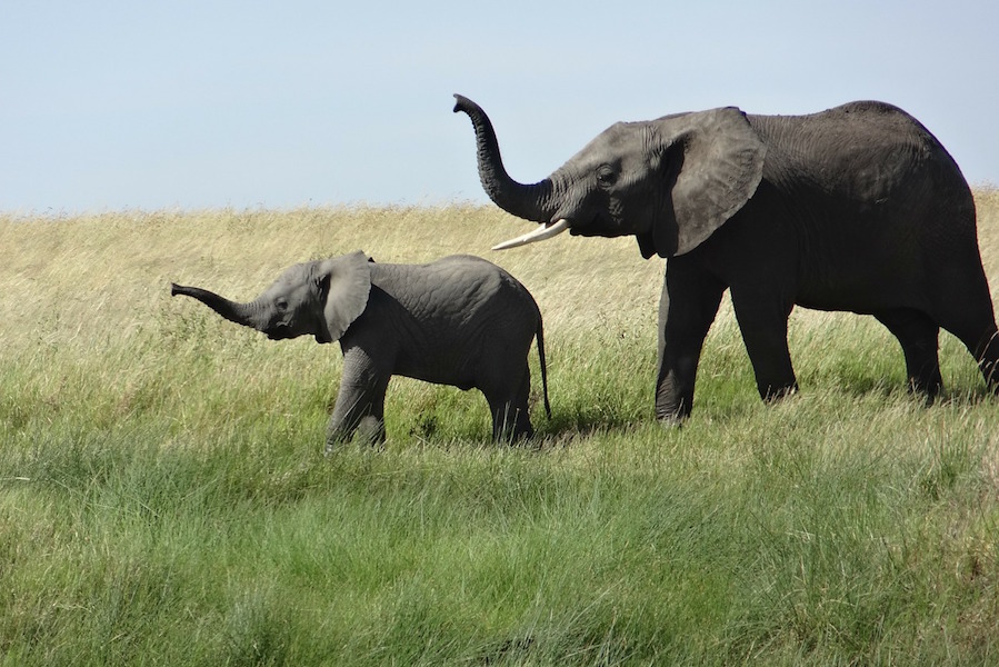
# Let's consider the following image of two African elephants, possible a mother and its cub, strolling in the savanna (under a Creative
# Commons license):
#
# 
# Let's convert this image into something the VGG16 model can read: the model was trained on images of size 224x244, preprocessed according
# to a few rules that are packaged in the utility function `keras.applications.vgg16.preprocess_input`. So we need to load the image, resize
# it to 224x224, convert it to a Numpy float32 tensor, and apply these pre-processing rules.
# In[27]:
from keras.preprocessing import image
from keras.applications.vgg16 import preprocess_input, decode_predictions
import numpy as np
# The local path to our target image
img_path = '/Users/fchollet/Downloads/creative_commons_elephant.jpg'
# `img` is a PIL image of size 224x224
img = image.load_img(img_path, target_size=(224, 224))
# `x` is a float32 Numpy array of shape (224, 224, 3)
x = image.img_to_array(img)
# We add a dimension to transform our array into a "batch"
# of size (1, 224, 224, 3)
x = np.expand_dims(x, axis=0)
# Finally we preprocess the batch
# (this does channel-wise color normalization)
x = preprocess_input(x)
# In[29]:
preds = model.predict(x)
print('Predicted:', decode_predictions(preds, top=3)[0])
#
# The top-3 classes predicted for this image are:
#
# * African elephant (with 92.5% probability)
# * Tusker (with 7% probability)
# * Indian elephant (with 0.4% probability)
#
# Thus our network has recognized our image as containing an undetermined quantity of African elephants. The entry in the prediction vector
# that was maximally activated is the one corresponding to the "African elephant" class, at index 386:
# In[30]:
np.argmax(preds[0])
# To visualize which parts of our image were the most "African elephant"-like, let's set up the Grad-CAM process:
# In[31]:
# This is the "african elephant" entry in the prediction vector
african_elephant_output = model.output[:, 386]
# The is the output feature map of the `block5_conv3` layer,
# the last convolutional layer in VGG16
last_conv_layer = model.get_layer('block5_conv3')
# This is the gradient of the "african elephant" class with regard to
# the output feature map of `block5_conv3`
grads = K.gradients(african_elephant_output, last_conv_layer.output)[0]
# This is a vector of shape (512,), where each entry
# is the mean intensity of the gradient over a specific feature map channel
pooled_grads = K.mean(grads, axis=(0, 1, 2))
# This function allows us to access the values of the quantities we just defined:
# `pooled_grads` and the output feature map of `block5_conv3`,
# given a sample image
iterate = K.function([model.input], [pooled_grads, last_conv_layer.output[0]])
# These are the values of these two quantities, as Numpy arrays,
# given our sample image of two elephants
pooled_grads_value, conv_layer_output_value = iterate([x])
# We multiply each channel in the feature map array
# by "how important this channel is" with regard to the elephant class
for i in range(512):
conv_layer_output_value[:, :, i] *= pooled_grads_value[i]
# The channel-wise mean of the resulting feature map
# is our heatmap of class activation
heatmap = np.mean(conv_layer_output_value, axis=-1)
# For visualization purpose, we will also normalize the heatmap between 0 and 1:
# In[32]:
heatmap = np.maximum(heatmap, 0)
heatmap /= np.max(heatmap)
plt.matshow(heatmap)
plt.show()
# Finally, we will use OpenCV to generate an image that superimposes the original image with the heatmap we just obtained:
# In[ ]:
import cv2
# We use cv2 to load the original image
img = cv2.imread(img_path)
# We resize the heatmap to have the same size as the original image
heatmap = cv2.resize(heatmap, (img.shape[1], img.shape[0]))
# We convert the heatmap to RGB
heatmap = np.uint8(255 * heatmap)
# We apply the heatmap to the original image
heatmap = cv2.applyColorMap(heatmap, cv2.COLORMAP_JET)
# 0.4 here is a heatmap intensity factor
superimposed_img = heatmap * 0.4 + img
# Save the image to disk
cv2.imwrite('/Users/fchollet/Downloads/elephant_cam.jpg', superimposed_img)
# 
# This visualisation technique answers two important questions:
#
# * Why did the network think this image contained an African elephant?
# * Where is the African elephant located in the picture?
#
# In particular, it is interesting to note that the ears of the elephant cub are strongly activated: this is probably how the network can
# tell the difference between African and Indian elephants.
#