/
cat2cat.Rmd
579 lines (480 loc) · 17.3 KB
/
cat2cat.Rmd
1
2
3
4
5
6
7
8
9
10
11
12
13
14
15
16
17
18
19
20
21
22
23
24
25
26
27
28
29
30
31
32
33
34
35
36
37
38
39
40
41
42
43
44
45
46
47
48
49
50
51
52
53
54
55
56
57
58
59
60
61
62
63
64
65
66
67
68
69
70
71
72
73
74
75
76
77
78
79
80
81
82
83
84
85
86
87
88
89
90
91
92
93
94
95
96
97
98
99
100
101
102
103
104
105
106
107
108
109
110
111
112
113
114
115
116
117
118
119
120
121
122
123
124
125
126
127
128
129
130
131
132
133
134
135
136
137
138
139
140
141
142
143
144
145
146
147
148
149
150
151
152
153
154
155
156
157
158
159
160
161
162
163
164
165
166
167
168
169
170
171
172
173
174
175
176
177
178
179
180
181
182
183
184
185
186
187
188
189
190
191
192
193
194
195
196
197
198
199
200
201
202
203
204
205
206
207
208
209
210
211
212
213
214
215
216
217
218
219
220
221
222
223
224
225
226
227
228
229
230
231
232
233
234
235
236
237
238
239
240
241
242
243
244
245
246
247
248
249
250
251
252
253
254
255
256
257
258
259
260
261
262
263
264
265
266
267
268
269
270
271
272
273
274
275
276
277
278
279
280
281
282
283
284
285
286
287
288
289
290
291
292
293
294
295
296
297
298
299
300
301
302
303
304
305
306
307
308
309
310
311
312
313
314
315
316
317
318
319
320
321
322
323
324
325
326
327
328
329
330
331
332
333
334
335
336
337
338
339
340
341
342
343
344
345
346
347
348
349
350
351
352
353
354
355
356
357
358
359
360
361
362
363
364
365
366
367
368
369
370
371
372
373
374
375
376
377
378
379
380
381
382
383
384
385
386
387
388
389
390
391
392
393
394
395
396
397
398
399
400
401
402
403
404
405
406
407
408
409
410
411
412
413
414
415
416
417
418
419
420
421
422
423
424
425
426
427
428
429
430
431
432
433
434
435
436
437
438
439
440
441
442
443
444
445
446
447
448
449
450
451
452
453
454
455
456
457
458
459
460
461
462
463
464
465
466
467
468
469
470
471
472
473
474
475
476
477
478
479
480
481
482
483
484
485
486
487
488
489
490
491
492
493
494
495
496
497
498
499
500
501
502
503
504
505
506
507
508
509
510
511
512
513
514
515
516
517
518
519
520
521
522
523
524
525
526
527
528
529
530
531
532
533
534
535
536
537
538
539
540
541
542
543
544
545
546
547
548
549
550
551
552
553
554
555
556
557
558
559
560
561
562
563
564
565
566
567
568
569
570
571
572
573
574
575
576
577
578
579
---
title: "Get Started"
author: "Maciej Nasinski"
date: "`r Sys.Date()`"
output:
rmarkdown::html_document:
theme: "spacelab"
highlight: "kate"
toc: true
toc_float: true
vignette: >
%\VignetteIndexEntry{Get Started}
%\VignetteEngine{knitr::rmarkdown}
%\VignetteEncoding{UTF-8}
---
```{r setup, include=FALSE}
knitr::opts_chunk$set(echo = TRUE)
knitr::opts_chunk$set(size = "tiny")
knitr::opts_chunk$set(message = FALSE)
knitr::opts_chunk$set(warning = FALSE)
```
## `cat2cat` procedure
The introduced `cat2cat` procedure was designed to offer an easy and clear interface to apply a mapping (transition) table which was provided by the data maintainer or built by a researcher. The objective is to unify an inconsistent coded categorical variable in a panel dataset, where a transition table is the core element of the process.
Examples of datasets with such inconsistent coded categorical variable are ISCO (The International Standard Classification of Occupations) or ICD (International Classification of Diseases) based one. The both classifications are regularly updated to adjust to e.g. new science achievements. More clearly we might image that e.g. new science achievements brings new occupations types on the market or enable recognition of new diseases types.
The categorical variable encoding changes are typically provided by datasets providers in the mapping (transition) table form, for each time point the changes occurred.
The mapping (transition) table is the core element of the procedure
A mapping table conveys information needed for matching all categories between two periods of time. More precisely it contains two columns where the first column contains old categories and the second column contains the new ones.
Sometimes a mapping (transition) table has to be created manually by a researcher.
The main rule is to replicate the observation if it could be assigned to a few categories.
More precisely for each observation we look across a mapping (transition) table to check how the original category could be mapped to the opposite period one. Then using simple frequencies or statistical methods to approximate weights (probabilities) of being assigned to each of them.
For each observation that was replicated, the probabilities have to add up to one.
The algorithm distinguishes different mechanics for panel data with and without unique identifiers.
## cat2cat function
The `cat2cat::cat2cat` function is the implementation of the `cat2cat` procedure.
The `cat2cat::cat2cat` function has three arguments `data`, `mappings`, and `ml`. Each
of these arguments is of a `list` type, wherein the
`ml` argument is optional. Arguments are separated to
identify the core elements of the `cat2cat` procedure.
Although this function seems
complex initially, it is built to offer a wide range of
applications for complex tasks. The function contains
many validation checks to prevent incorrect usage.
The function has to be applied iteratively for each two neighboring periods of a panel dataset.
The `cat2cat::prune_c2c` function could be needed to limit growing number of replications.
## Core elements
There are 3 important elements:
1. Mapping (Transition) table, possibly a few for longer panels. Typically provided by the data maintainers like a statistical office.
2. Type of the data - panel dataset with unique identifiers vs panel dataset without unique identifiers and aggregate data vs non-aggragate data.
3. Direction of a mapping process, forward or backward - a new or an old encoding as a base one.
## Data
`occup` dataset is an example of unbalance panel dataset.
This is a simulated data although there are applied a real world characteristics from national statistical office survey.
The original survey is anonymous and take place **every two years**.
`trans` mapping (transition) table contains mappings between old (2008) and new (2010) occupational codes. This table could be used to map encodings in both directions.
```{r, message=FALSE, warning=FALSE}
library("cat2cat")
library("dplyr")
data("occup", package = "cat2cat")
data("trans", package = "cat2cat")
occup_2006 <- occup[occup$year == 2006, ]
occup_2008 <- occup_old <- occup[occup$year == 2008, ]
occup_2010 <- occup_new <- occup[occup$year == 2010, ]
occup_2012 <- occup[occup$year == 2012, ]
```
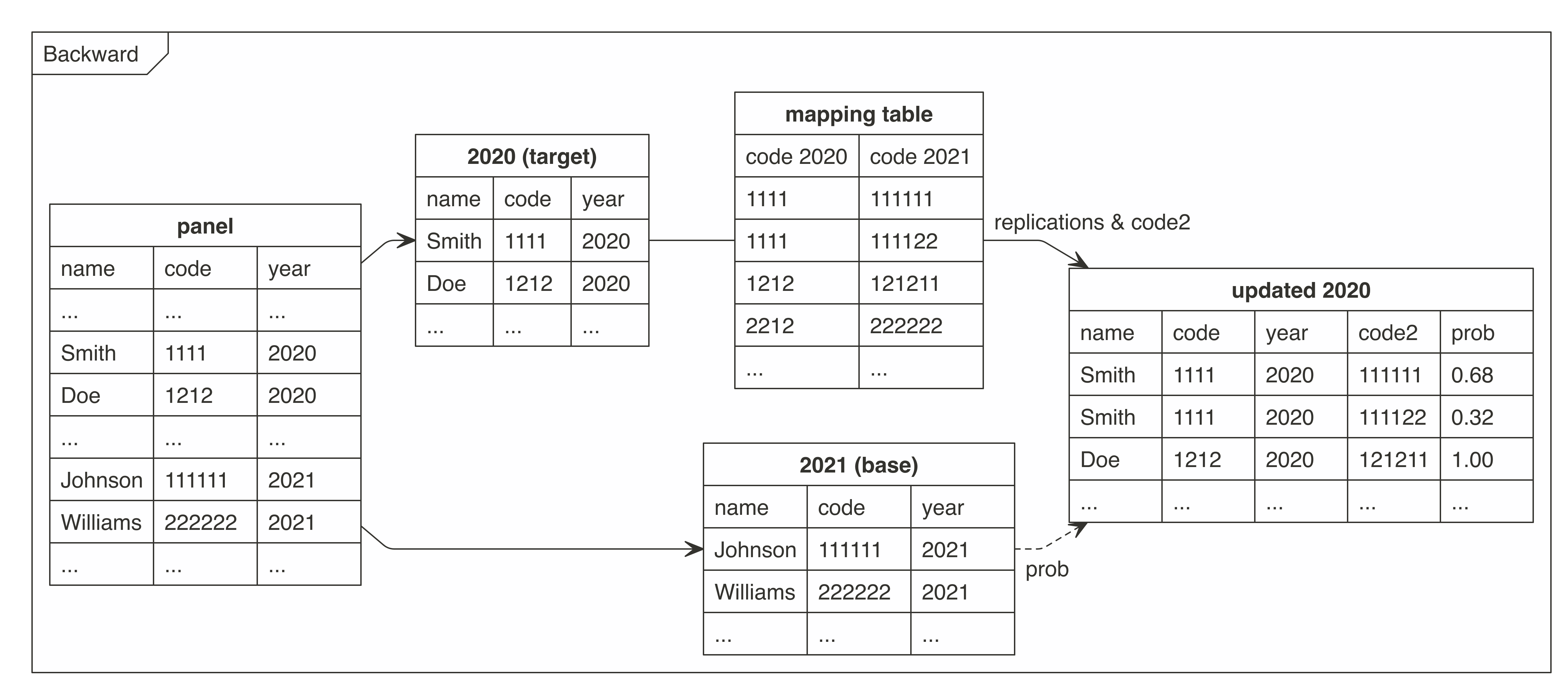
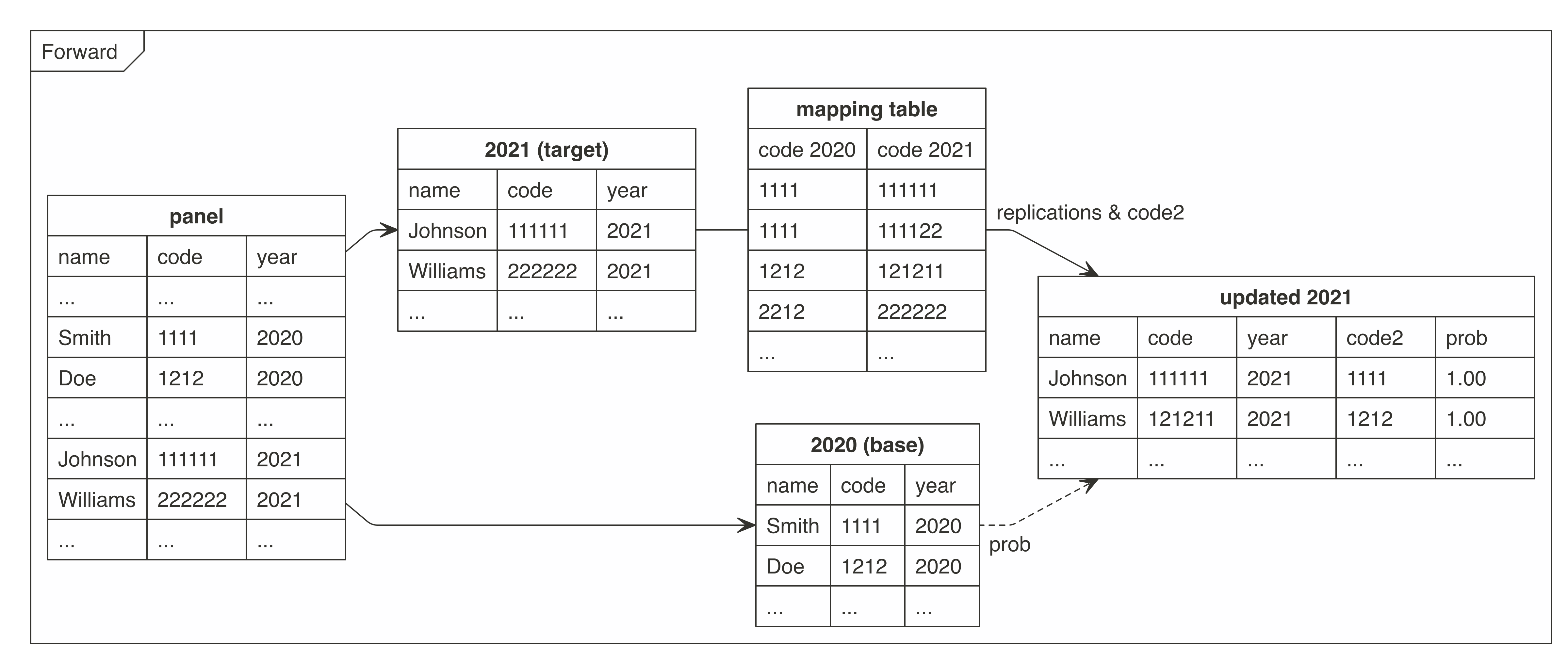
## Dataset without unique identifiers
There were prepared two graphs for forward and backward mapping.
These graphs present how the `cat2cat::cat2cat` procedure works, in this case under a panel dataset without the unique identifiers and only two periods.
### Example - 2 periods
```{r}
## cat2cat
occup_simple <- cat2cat(
data = list(
old = occup_old, new = occup_new, cat_var = "code", time_var = "year"
),
mappings = list(trans = trans, direction = "backward")
)
## with informative features it might be usefull to run ml algorithm
## currently knn, lda and rf (randomForest), could be a few at once
## where probability will be assessed as fraction of closest points.
occup_2 <- cat2cat(
data = list(
old = occup_old, new = occup_new,
cat_var = "code", time_var = "year"
),
mappings = list(trans = trans, direction = "backward"),
ml = list(
data = occup_new,
cat_var = "code",
method = "knn",
features = c("age", "sex", "edu", "exp", "parttime", "salary"),
args = list(k = 10)
)
)
```
`plot_c2c` offers a summary of the replication process.
```{r}
# summary_plot
plot_c2c(occup_2$old, type = c("both"))
```
Example for the 2 period panel dataset.
```{r}
# mix of methods
occup_2_mix <- cat2cat(
data = list(
old = occup_old, new = occup_new,
cat_var = "code", time_var = "year"
),
mappings = list(trans = trans, direction = "backward"),
ml = list(
data = occup_new,
cat_var = "code",
method = c("knn", "rf", "lda"),
features = c("age", "sex", "edu", "exp", "parttime", "salary"),
args = list(k = 10, ntree = 50)
)
)
# cross all methods and subset one highest probability category for each subject
occup_old_mix_highest1 <- occup_2_mix$old %>%
cross_c2c(.) %>%
prune_c2c(., column = "wei_cross_c2c", method = "highest1")
```
Correlations between different methods of assesing weights are presented.
```{r}
# correlation between ml models and simple fequencies
occup_2_mix$old %>%
select(wei_knn_c2c, wei_rf_c2c, wei_lda_c2c, wei_freq_c2c) %>%
cor()
```
### Example - More than 2 periods
When we have to map more than 2 time points, then
cat2cat has to be used iteratively.
However when only three periods have to be mapped, the middle one
could be used as the base one.
If we have to apply many different mapping (transition) tables over time then pruning methods could be needed to limit the exponentially growing number of replications.
Such pruning methods are used to remove some of the replications, for example, leaving only
one observation with the highest probability for each observation
replication. Another strategy might be removing the zero probability
replications. As such, pruning methods could be used before transferring a
dataset to the next iteration to reduce the problem of the exponentially
growing number of observations.
Example with 4 period and only one mapping table:
#### Backward
Unification Process:
```{r}
# from 2010 to 2008
occup_back_2008_2010 <- cat2cat(
data = list(
old = occup_2008, new = occup_2010,
cat_var = "code", time_var = "year"
),
mappings = list(trans = trans, direction = "backward")
)
# optional, give more control
# the counts could be any of wei_* or their combination
freqs_df <-
occup_back_2008_2010$old[, c("g_new_c2c", "wei_freq_c2c")] %>%
group_by(g_new_c2c) %>%
summarise(counts = round(sum(wei_freq_c2c)))
# from 2008 to 2006
occup_back_2006_2008 <- cat2cat(
data = list(
old = occup_2006,
new = occup_back_2008_2010$old,
cat_var_new = "g_new_c2c",
cat_var_old = "code",
time_var = "year"
),
mappings = list(
trans = trans, direction = "backward",
freqs_df = freqs_df
)
)
o_2006_new <- occup_back_2006_2008$old
# or occup_back_2006_2008$new
o_2008_new <- occup_back_2008_2010$old
o_2010_new <- occup_back_2008_2010$new
# use ml argument when applied ml models
o_2012_new <- dummy_c2c(occup_2012, "code")
final_data_back <- do.call(
rbind,
list(o_2006_new, o_2008_new, o_2010_new, o_2012_new)
)
```
Valiation of global counts and per variable level counts:
```{r}
# We persist the number of observations
counts_new <- final_data_back %>%
cross_c2c() %>%
group_by(year) %>%
summarise(
n = as.integer(round(sum(wei_freq_c2c))),
n2 = as.integer(round(sum(wei_cross_c2c)))
)
counts_old <- occup %>%
group_by(year) %>%
summarise(n = n(), n2 = n(), .groups = "drop")
identical(counts_new, counts_old)
# counts per each level
counts_per_level <- final_data_back %>%
group_by(year, g_new_c2c) %>%
summarise(n = sum(wei_freq_c2c), .groups = "drop") %>%
arrange(g_new_c2c, year)
```
#### Forward
Unification Process:
A few categories levels are not in the trans table, lacking levels `setdiff(c(occup_2010$code, occup_2012$code), trans$new)`.
We could solve it by adding a "no_cat" level for each of them in the `trans` table.
```{r}
trans2 <- rbind(
trans,
data.frame(
old = "no_cat",
new = setdiff(
c(occup_2010$code, occup_2012$code),
trans$new
)
)
)
```
Of course the best solution will be to get these mappings from the data provider
```{r}
# from 2008 to 2010
occup_for_2008_2010 <- cat2cat(
data = list(
old = occup_2008, new = occup_2010,
cat_var = "code", time_var = "year"
),
mappings = list(trans = trans2, direction = "forward")
)
# optional, give more control
# the counts could be any of wei_* or their combination
freqs_df <-
occup_for_2008_2010$new[, c("g_new_c2c", "wei_freq_c2c")] %>%
group_by(g_new_c2c) %>%
summarise(counts = round(sum(wei_freq_c2c)))
# from2010 to 2012
occup_for_2010_2012 <- cat2cat(
data = list(
old = occup_for_2008_2010$new,
new = occup_2012,
cat_var_old = "g_new_c2c",
cat_var_new = "code",
time_var = "year"
),
mappings = list(
trans = trans2, direction = "forward",
freqs_df = freqs_df
)
)
# use ml argument when applied ml models
o_2006_new <- dummy_c2c(occup_2006, "code")
o_2008_new <- occup_for_2008_2010$old
o_2010_new <- occup_for_2008_2010$new # or occup_for_2010_2012$old
o_2012_new <- occup_for_2010_2012$new
final_data_for <- do.call(
rbind,
list(o_2006_new, o_2008_new, o_2010_new, o_2012_new)
)
```
Valiation of global counts and per variable level counts.
```{r}
# We persist the number of observations
counts_new <- final_data_for %>%
cross_c2c() %>%
group_by(year) %>%
summarise(
n = as.integer(round(sum(wei_freq_c2c))),
n2 = as.integer(round(sum(wei_cross_c2c)))
)
counts_old <- occup %>%
group_by(year) %>%
summarise(n = n(), n2 = n(), .groups = "drop")
identical(counts_new, counts_old)
# counts per each level
counts_per_level <- final_data_for %>%
group_by(year, g_new_c2c) %>%
summarise(n = sum(wei_freq_c2c), .groups = "drop") %>%
arrange(g_new_c2c, year)
```
#### Backward and ML
Unification Process:
```{r}
ml_setup <- list(
data = dplyr::bind_rows(occup_2010, occup_2012),
cat_var = "code",
method = c("knn"),
features = c("age", "sex", "edu", "exp", "parttime", "salary"),
args = list(k = 10)
)
mappings <- list(trans = trans, direction = "backward")
# ml model performance check
print(cat2cat_ml_run(mappings, ml_setup))
# from 2010 to 2008
occup_back_2008_2010 <- cat2cat(
data = list(
old = occup_2008, new = occup_2010,
cat_var = "code", time_var = "year"
),
mappings = mappings,
ml = ml_setup
)
# from 2008 to 2006
occup_back_2006_2008 <- cat2cat(
data = list(
old = occup_2006,
new = occup_back_2008_2010$old,
cat_var_new = "g_new_c2c",
cat_var_old = "code",
time_var = "year"
),
mappings = mappings,
ml = ml_setup
)
o_2006_new <- occup_back_2006_2008$old
# or occup_back_2006_2008$new
o_2008_new <- occup_back_2008_2010$old
o_2010_new <- occup_back_2008_2010$new
o_2012_new <- dummy_c2c(occup_2012, cat_var = "code", ml = c("knn"))
final_data_back_ml <- do.call(
rbind,
list(o_2006_new, o_2008_new, o_2010_new, o_2012_new)
)
```
Valiation of global counts and per variable level counts.
```{r}
counts_new <- final_data_back_ml %>%
cross_c2c() %>%
group_by(year) %>%
summarise(
n = as.integer(round(sum(wei_freq_c2c))),
n2 = as.integer(round(sum(wei_cross_c2c))),
.groups = "drop"
)
counts_old <- occup %>%
group_by(year) %>%
summarise(n = n(), n2 = n(), .groups = "drop")
identical(counts_new, counts_old)
# counts per each level
counts_per_level <- final_data_back_ml %>%
group_by(year, g_new_c2c) %>%
summarise(n = sum(wei_freq_c2c), .groups = "drop") %>%
arrange(g_new_c2c, year)
```
Possible processing:
```{r}
ff <- final_data_back_ml %>%
split(.$year) %>%
lapply(function(x) {
x %>%
cross_c2c() %>%
prune_c2c(column = "wei_cross_c2c", method = "highest1")
}) %>%
bind_rows()
all.equal(nrow(ff), sum(final_data_back_ml$wei_freq_c2c))
```
## Regression
The replication process is neutral for calculating at least the first 2 central moments for all variables.
This is because for each observation which was replicated, probabilities sum to one.
If we are removing non-zero probability observations then replication probabilities have to be reweighed to still sum to one.
Important note is that removing non zero probability observations should be done only if needed, as it impact the counts of categorical variable levels. More preciously removing non-zero weights will influence the regression model if we will use the unified categorical variable.
### Regression - neutral impact
The next 3 regressions have the same results.
```{r}
## orginal dataset
lms2 <- lm(
I(log(salary)) ~ age + sex + factor(edu) + parttime + exp,
data = occup_old,
weights = multiplier
)
summary(lms2)
## using one highest cross weights
## cross_c2c to cross differen methods weights
## prune_c2c
## highest1 leave only one the highest probability obs for each subject
occup_old_2 <- occup_2$old %>%
cross_c2c(., c("wei_freq_c2c", "wei_knn_c2c"), c(1, 1) / 2) %>%
prune_c2c(., column = "wei_cross_c2c", method = "highest1")
lms <- lm(
I(log(salary)) ~ age + sex + factor(edu) + parttime + exp,
data = occup_old_2,
weights = multiplier
)
summary(lms)
## we have to adjust size of stds
## as we artificialy enlarge degrees of freedom
occup_old_3 <- occup_2$old %>%
prune_c2c(method = "nonzero") # many prune methods like highest
lms_replicated <- lm(
I(log(salary)) ~ age + sex + factor(edu) + parttime + exp,
data = occup_old_3,
weights = multiplier * wei_freq_c2c
)
# Adjusted R2 is meaningless here
lms_replicated$df.residual <-
nrow(occup_old) - length(lms_replicated$assign)
suppressWarnings(summary(lms_replicated))
```
### Regression with unified variable
Example regression model with usage of the unified variable (`g_new_c2c`).
A separate model for each occupational group.
```{r}
formula_oo <- formula(
I(log(salary)) ~ age + sex + factor(edu) + parttime + exp + factor(year)
)
oo <- final_data_back %>%
prune_c2c(method = "nonzero") %>% # many prune methods like highest
group_by(g_new_c2c) %>%
filter(n() >= 15) %>%
do(
lm = tryCatch(
summary(lm(formula_oo, ., weights = multiplier * wei_freq_c2c)),
error = function(e) NULL
)
) %>%
filter(!is.null(lm))
head(oo)
oo$lm[[2]]
```
## Manual mappings
`cat2cat_agg` is mainly useful for aggregate datasets.
```{r}
library("cat2cat")
data("verticals", package = "cat2cat")
agg_old <- verticals[verticals$v_date == "2020-04-01", ]
agg_new <- verticals[verticals$v_date == "2020-05-01", ]
## cat2cat_agg - could map in both directions at once although
## usually we want to have old or new representation
agg <- cat2cat_agg(
data = list(
old = agg_old,
new = agg_new,
cat_var = "vertical",
time_var = "v_date",
freq_var = "counts"
),
Automotive %<% c(Automotive1, Automotive2),
c(Kids1, Kids2) %>% c(Kids),
Home %>% c(Home, Supermarket)
)
## possible processing
library("dplyr")
agg %>%
bind_rows() %>%
group_by(v_date, vertical) %>%
summarise(
sales = sum(sales * prop_c2c),
counts = sum(counts * prop_c2c),
v_date = first(v_date),
.groups = "drop"
)
```
## Dataset with unique identifiers
If the panel dataset is balanced so contains consistent subjects id's for each period then we could match some of the categories directly.
Unfortunately we have to assume that a subject could not change the category level over time.
```{r}
library(cat2cat)
## the ean variable is a unique identifier
data("verticals2", package = "cat2cat")
vert_old <- verticals2[verticals2$v_date == "2020-04-01", ]
vert_new <- verticals2[verticals2$v_date == "2020-05-01", ]
## get mapping (transition) table
trans_v <- vert_old %>%
inner_join(vert_new, by = "ean") %>%
select(vertical.x, vertical.y) %>%
distinct()
```
```{r}
## cat2cat
## it is important to set id_var as then we merging categories 1 to 1
## for this identifier which exists in both periods.
verts <- cat2cat(
data = list(
old = vert_old, new = vert_new, id_var = "ean",
cat_var = "vertical", time_var = "v_date"
),
mappings = list(trans = trans_v, direction = "backward")
)
```