Exercise9.md

View this on Github View this in "作业部落"

Exercise 9: Chaos in the Driven Nonlinear Pendulum

王世兴 2013301020050

---

Level 1
Construct Poincare sections for various cases and compare them with Figure 3.9 in Reference [1]

---

Level 2
Investigate how a strange attractor is altered by small changes in one of these pendulum parameters.
Investigate the bifurcation diagrams found for the pendulum with other values of the drive frequency and damping parameter.

---

Abstract

Chaos is an unpredictable phenomenon in a classical system domineered by the determinnistic classical mechanics. Poincare section and the bifurcation diagram are two ways to present and investigate chaos. The program calculating chaos and showing the plot of angular displacement versus time, the plot of Poincare sections and bifurcation diagram are presented. Also various parameters of the driven amplitude and frequency are tested to investigate the parameter sensitivity of the Poincare section and bifurcation diagram.

Background

Driven Nonlinear Pendulum and Chaos

In this report we only discuss a model where the pendulum is domineered by a sinusoidal external driving force and a frinction force proportional to the angular speed, while the restoring force is also a sinuous function of angular displacement.[1]
$$\frac{d^2\theta}{dt^2}=-\frac{g}{l}\text{sin}\theta-q\frac{d\theta}{dt}+F_D\text{sin}(\Omega_Dt)$$
As usual we introduce the first derivative of angular displacement and rewrite it as two first-order differential equations
$$ \begin{array}{ll} \frac{d\omega}{dt}&=-\frac{g}{l}\text{sin}\theta-q\omega+F_D\text{sin}(\Omega_Dt)\\frac{d\theta}{dt}&=\omega \end{array} $$
And as we will see in the "Result" section, under some $F_D$ choices the system will show a weird behavior. This weirdness is called "chaos", where a slight difference of the initial conditions may yield dramatically different results, even if this system is deterministic. Just as Edward Lorenz puts it, "When the present determines the future, but the approximate present does not approximately determine the future."

Qualitative and Stability Theory

By work of Liouville, it is well known that most differential equations could not be solved with elementary integal. Then the question of interest becomes whether we can judge the properties of the solution by the equations themselves. The French mathematicist Poincare came up with the qualitative theory and the Russian mathematicist Liapunov established the stability theory separately and contemporarily. [2]

The stability of the solution to an equation is defined as: for equations
$$\frac{d\vec x}{dt}=f(t,\vec x)$$
and $f(t,\vec x)$ satisfies the Lipschitz condition, for the initial condition $(t_0,\vec x_0)$ the solution $\vec x=\vec \varphi(t,t_0,\vec x_0)$, for any given $\epsilon>0,t_0>0$, there exist $\delta(\epsilon,t_0)>0$, such that $$||\vec x_0-\vec x_1||<\delta$$ $$||\vec x(t,t_0,\vec x_0)-\vec \varphi(t,t_0,\vec x_1)||<\epsilon$$

Figuratively speaking, the stability means when the initial conditions deviate a little amount, the amount of the variance of the solution is also small.

Liapunov also gived methods to determine whether an equation is stable. The commonly-discussed Liapunov's second method uses a so-called Liapunov funciton $V(x)$, judging the stability by the sign of the derivative $dV(x)/dx$.

Phase Plain, Phase Diagram, and Phase Trajectory

Simultaneous differential equations are called a plain autonumous system
$$\begin{matrix}\dot{x}=P(x,y)\\dot{y}=Q(x,y)\end{matrix}$$
such that the funcitons $P(x,y),Q(x,y)$ satisfy the condition for the unique existence theorem.[2] In our problem the function becomes $\theta(t)$ and $\omega(t)$. They are assumed independent also physically $\omega(t)$ is the time derivative of $\theta(t)$.

We define the xOy plain (the $\theta O\omega$ plain in our problem) as the phase plain. And the solution to the differential equations $x=x(t),y=y(t)$ (in our problem $\theta(t)$ and $\omega(t)$) in the plain are called the phase trajectories. The trajectory clusters are called the phase diagram.

Poincare section and Bifurcation Diagram

Once we get the phase trajectories, some interesting and exciting tricks could be used to find more on the properties of chaos.

If we only show the points at the same phase of the driving force, the result is called the Poincare section. Obviously if there is no chaos the Poincare section would be a single point in the phase space. However, for chaotic system the Poincare section would show a fractal behavior.

To determine the critical point where the chaotic behavior appears and changes, we observe the angular displacement on the same value of the driving force, which is called bifuraction diagram.

Result

The source code is open on Github. Details of the codes will be discussed in the following section.

$\theta(t)$ plot and Phase Trajectory

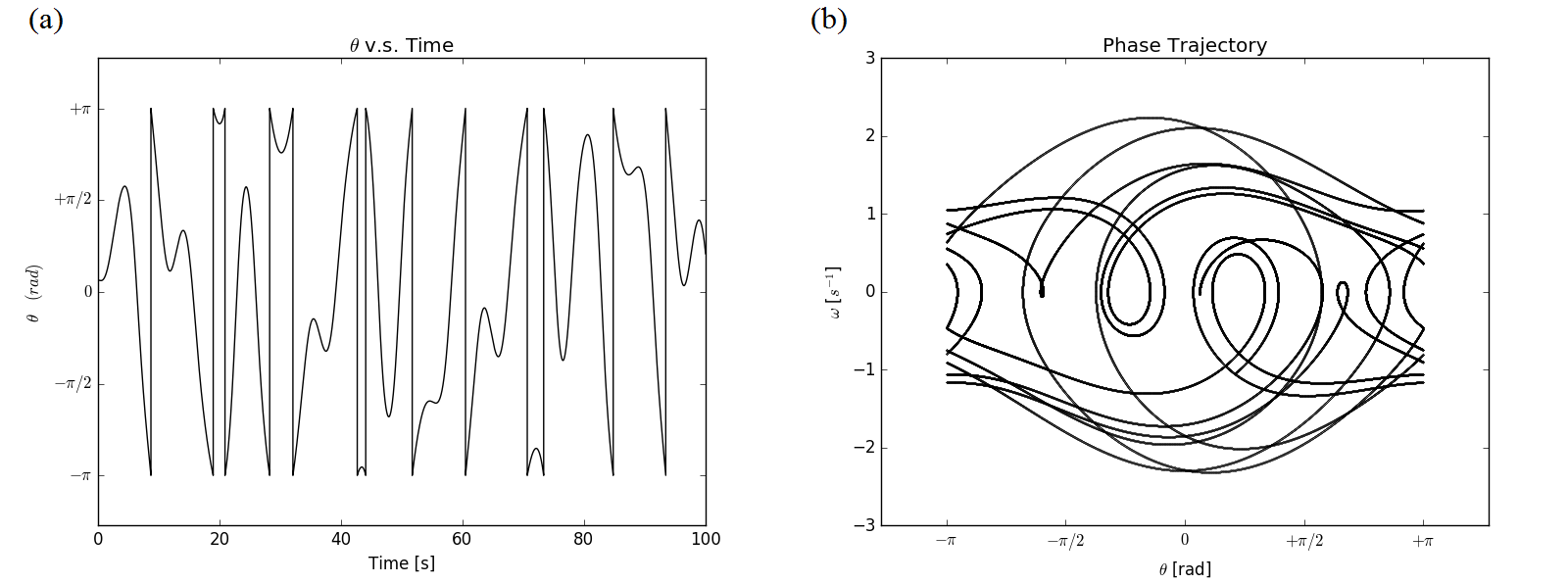
Figure 9.1 The $\theta(t)$ plot (a) and phase trajectory (b), with l=g=9.8, q=0.5, $F_D$=1.2

Level 1: Poincare Sections

The definition of Poincare sections and methods to obtain it is introduced in the Background section, and we choose four phases at $0$, $\pi/4$, $\pi/2$, $3\pi/4$ and plot the Poincare section separately (Figure 9.2) and altogether (Figuer 9.3). It is noticable the similarity between the superposition of the Poincare sections and the phase trafjectory. We can imagine as the phase chosen approachs the whole period, the superposition of Poincare section naturally becomes the phase trajectory.

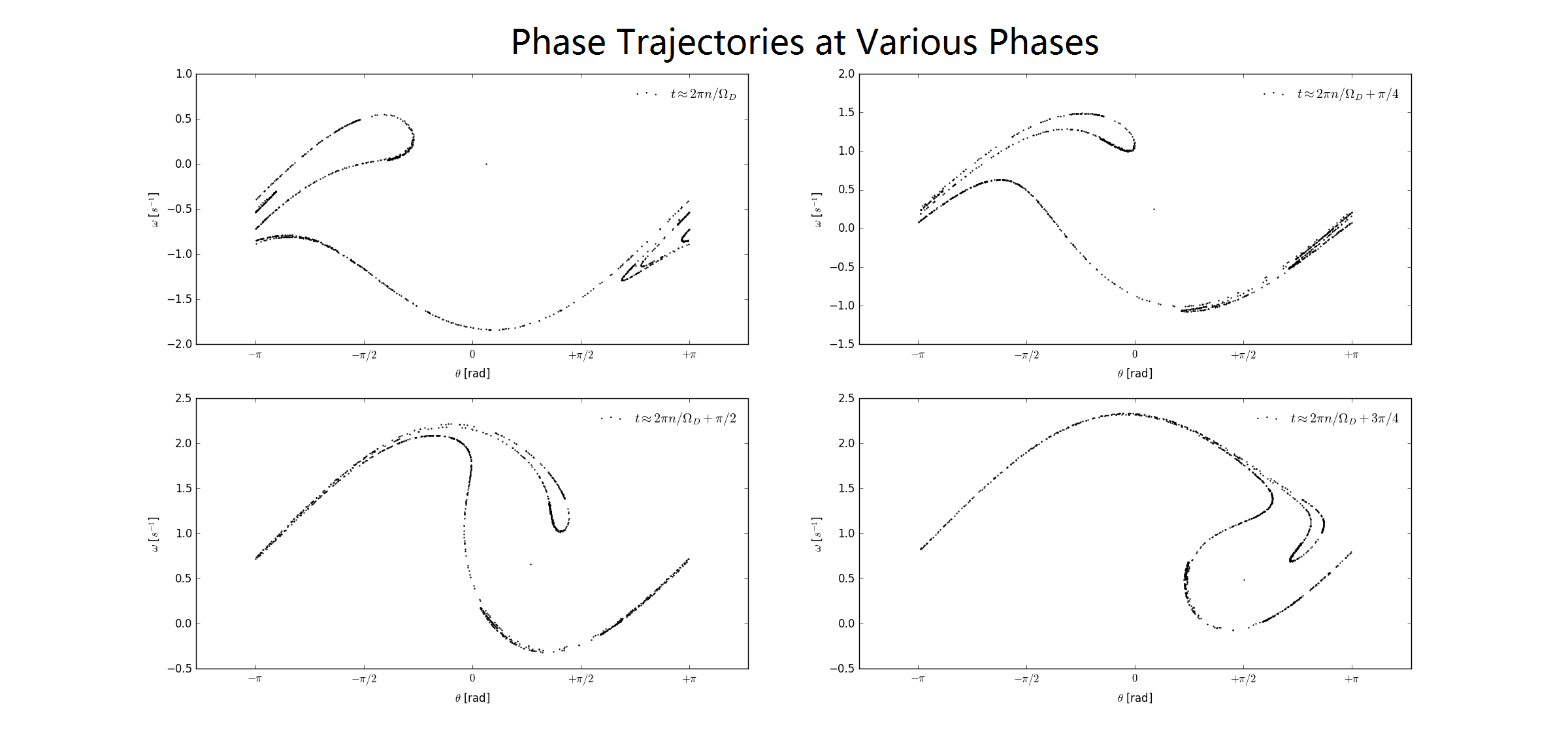
Figure 9.2 Poincare sections at four different phases.

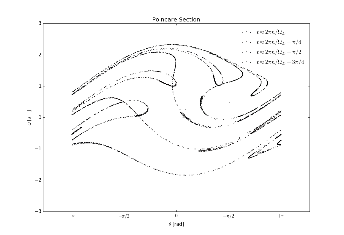
Figure 9.3 Superposition of the four Poincare section plots.

And an interesting property that the Poincare section possesses is the fractal structure. We can zoom up a certain region of the Poincare section with phase zero and see (Figure 9.4) that there are countably infinite points in every region and they share a property of self-similarity (although not exactly the same). This is a typical fractal structure.

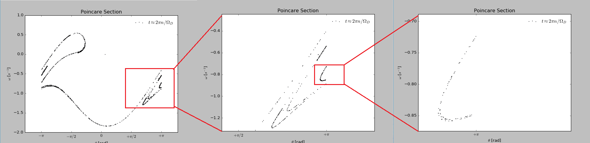
Figure 9.4 Fractal structure of Poincare section.

Level 2: Bifurcation Diagram with Various Parameters

The bifurcation diagram is obtained according to the guidance from Reference [1], discussed in detail in the following

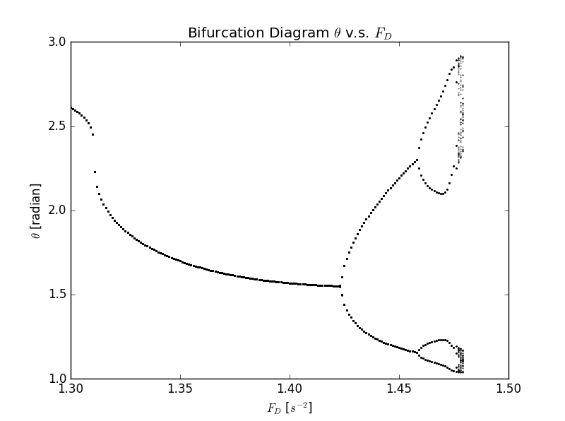
Figure 9.5 Bifurcation Diagram with $\Omega_D=2/3$, $q=1/2$.

And we tried several different choices of the frequency of the driving force (in Figure 9.5) and the friction coefficient (in Figure 9.6)

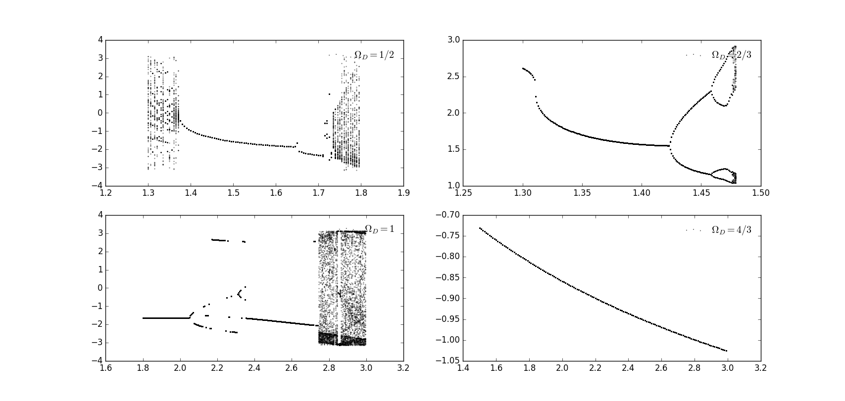
Figure 9.5 Bifurcation diagram with $\Omega_D=1/2$ (upper left), $\Omega_D=2/3$ (upper right),$\Omega_D=1$ (lower left), $\Omega_D=4/3$ (lower right).

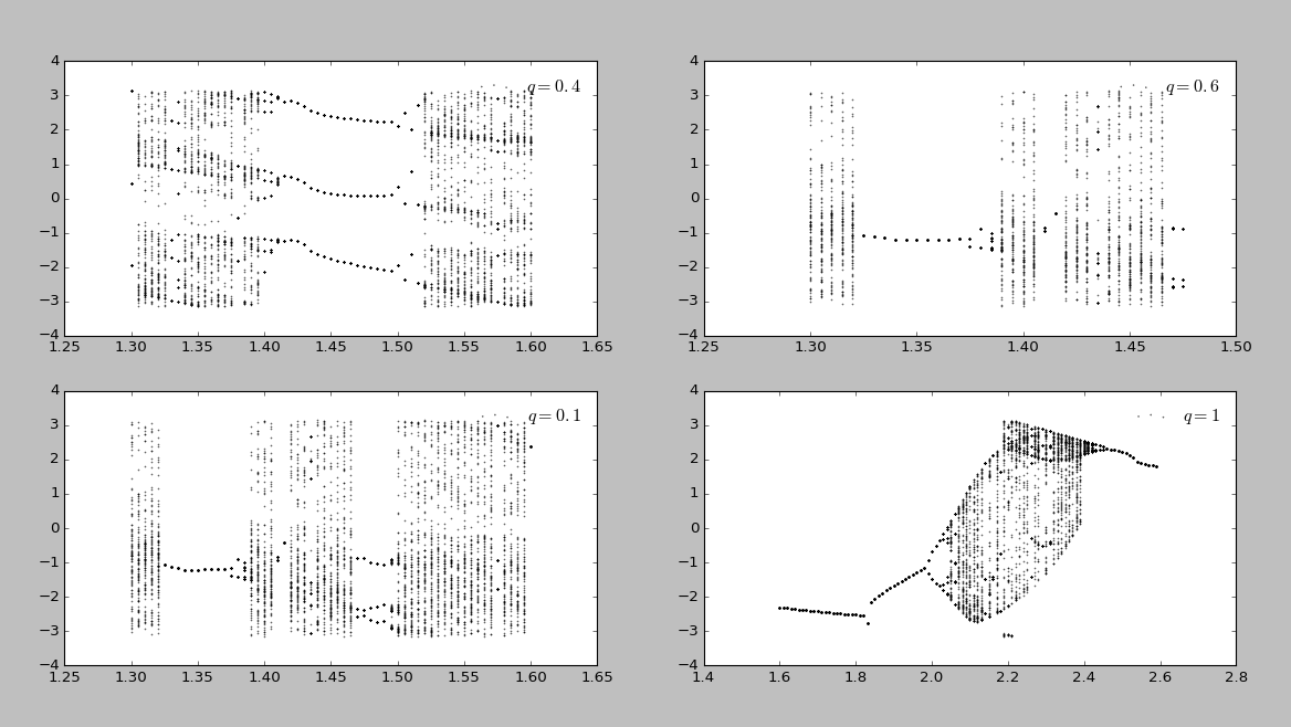
Figure 9.6 Bifurcation diagram with $q=0.4$ (upper left), $q=0.6$ (upper right),$q=0.1$ (lower left), $q=1$ (lower right). The x coordinate is driving force amplitude (unit: $s^{-2}$), and the y coordinate is angular displacement (unit: radian)

We can see that chaos happen at a relatively large range of the choice of parameters. However, we can not find an analytical expression for the relationship between the number of points of $\theta$ at a certain $F_D$. This is an obvious drawback of numerical simulation discussed by Meerschaert. [3]

Discussion: Main Features of the Code

• Subtle time step length.
  In order to meet the requirement that we can observe the angular dislplacement in phase with the driving force we adjust the step length of the root-finding program to be an integal division of $\pi$

• Reshape of the data with mode $2\pi$

• Scatter Diagram.

Reference

1. Giodano, N.J., Nakanishi, H. Computational Physics. Tsinghua University Press, December 2007

2. Differential Equation Group of Northeast University. Ordinary Differential Equation, Second Edition. Higher Education Press, April 2005.

3. Meerschaert, 《数学建模与分析方法（第一版）》，机械工业出版社，2009年5月1日