RTX & CrowdNav Getting Started Guide
In this document we give a brief introduction to two two artifacts we have bundled together.
- CrowdNav - a simulation based on SUMO and TraCI that implements a custom router that can be configured using kafka messages or local JSON config on the fly while the simulation is running. Also runtime data is send to a kafka queue to allow stream processing and logger locally to CSV.
- RTX - a tool that allows for self-adaptation based on analysis of real time (streaming) data. RTX is particularly useful in analyzing operational data in a Big Data environment.
To simplify working with the artifacts, we offer multiple ways to run them and
also worked hard to allow a cross-platform usage on Windows, Linux and MacOS.
You have the following options when running the artifact:
The easiest way to have a look into the tool and what it is doing is to use our provided docker containers.
To use this approach follow the following instructions:
-
Get Docker running on your OS - Click for Instructions
-
The next step is to run Kafka as we use this instance for CrowdNav and RTX.
To do this execute the following command. It will start pre-configured kafka server with the hostname kafka and open the relevant ports.docker run --name kafka --hostname kafka -p 2181:2181 -p 9092:9092 --env ADVERTISED_HOST=kafka --env ADVERTISED_PORT=9092 spotify/kafka -
Once kafka is running we start CrowdNav to run the simulation. Here we offer two options:
- console mode - where CrowdNav works using console output as long as the container is alive.
docker run -it --link kafka:kafka starofall/crowdnav- gui mode - to see what CrowdNav is doing, this mode allows the user to see the SUMO-GUI graphical user interface using VNC.
docker run -it -p 6080:6080 --link kafka:kafka starofall/crowdnavgui-dockerOnce the container is running, open the browser to either
localhost:6080or(IP of your Boot2Docker):6080.
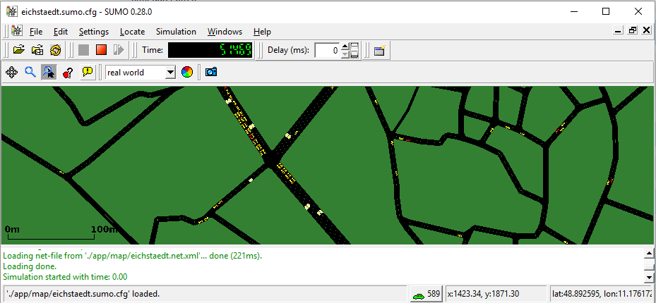
Here you should see the desktop transmitted over vnc. Once you click the shortcut on the desktop, CrowdNav boots up and the simulation can be started using the play button.
If you want to take a deeper look into the tool and also want to play around with the configuration files, we provide a VM image that is already pre-configured to have all dependencies and software installed.
- Download and import the provided VHD file into your VM provider. Give the VM at least 1GB of RAM to run.
- Once the VM is running you have to start kafka using the icon on the desktop. Always click on “open in terminal” and if asked the password is “seam”.
- RTX and CrowdNav are already provided on the desktop with additional tooling scripts.
It is recommended to read the readme files provided in these folders. Also run the update scripts to assure you are using the most recent version. - You can run CrowdNav without doing experiments using RTX, but not vice versa.
If you want to use the tool more extensively it is recommended to install it locally.
To do so follow these instructions:
- For Kafka we also propose to use the docker container as described in the text above.
When you are using Boot2Docker you might need to add an entry to your hosts file to link(IP of your Boot2Docker)to the hostnamekafka.
If you want to install Kafka manually, please read these instructions. - Next step is to install SUMO. The instructions for this are depending on your operating system:
- Official Instructions
- Please make sure you at least have version 0.27 installed and the env variable
SUMO_HOMEis set to the sumo folder. - If your distro does offer an older version than 0.27, you have to build SUMO from source using this commands:
sudo apt-get install -y build-essential git libxerces-c-dev
sudo mkdir -p /opt && sudo cd /opt
sudo git clone https://github.com/radiganm/sumo.git
sudo cd /opt/sumo && sudo ./configure
sudo cd /opt/sumo && sudo make
sudo cd /opt/sumo && sudo make install
export SUMO_HOME=/opt/sumo
- Extract CrowdNav from the archive or download the recent source code from the CrowdNav Repository.
- Make sure you have
python 2.7installed. - Run the following commands within the CrowdNav folder:
sudo apt-get install libfreetype6-dev libpng-dev # needed for older distros sudo python setup.py install - Now you should be able to run
python run.pyand see the SUMO interface where you have to start the simulation. - Extract RTX from the archive or download the recent source code from the RTX Repository.
- On Windows you have to manually install
numpyandscipy. We provide compiled versions of these libraries and an install script for this attools/winlibs/install.bat. - Also on older distros installing
numpyandscipycan be challenging. Please look here and here for more information. - Run the following commands within the RTX folder:
sudo python setup.py install - If everything worked, you can now run experiments - e.g. by using:
python rtx.py start examples/crowdnav-sequential
- CrowdNav will not send messages for the first 1000 ticks to let the system stabilize, so please be patient.
- Running a RTX experiment that is using Spark can also take some time to bootup.
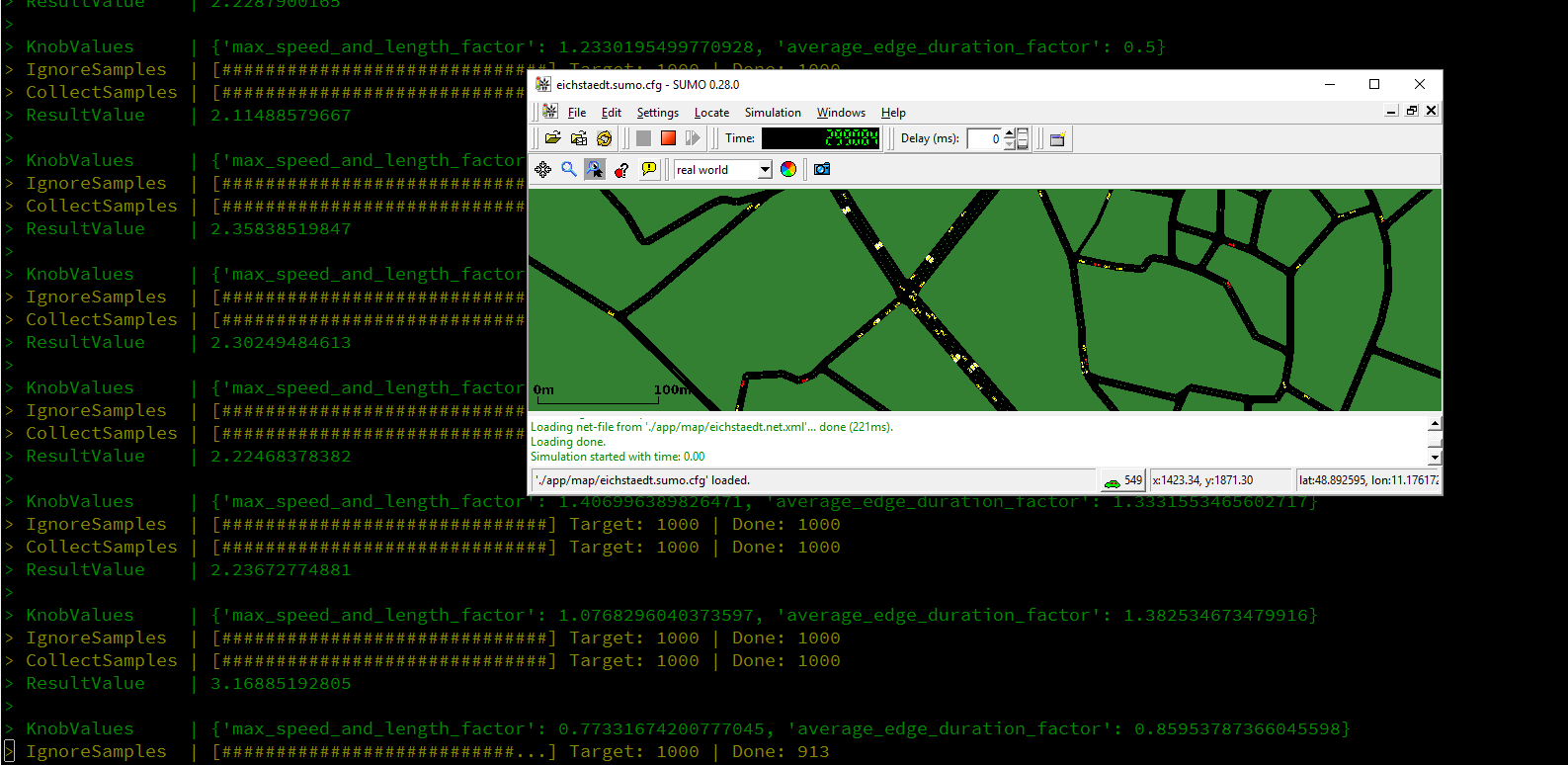
Once you have the system installed you can do the following things:
- Run the GUI application and inspect that there are cars that are red (controlled by us) and green (send to exploration by us).
- See where traffic jams happen and how good the red cars are avoiding them over the time.
- Modify the source code of the CustomRouter.py to your own routing algorithm.
- If you set
kafkaUpdatestoFalsein theConfig.pyfile you can adjust the router with theknobs.jsonfile.- Do not forget to revert this if you want to use RTX for running experiments.
- Use
forever.pyto run the simulation in the background forever. - Use
parallel.py #nto spawn n processes and let them run for 10.000 ticks for benchmarks and data generation.
-
Try out all the provided examples (see list of folders starting with crowdnav) by issuing
python rtx.py start [folder name] -
Look at the auto generated diagrams for the experiments
-
Regenerate the diagrams from already run experiments by issuing
python rtx.py report [folder name] -
Change variables in the different
definition.pyto run other experiments. -
Implement a custom target system and optimize it.
RTX has the following abstractions that can be implemented for any given service:
- PreProcessor - Is used to reduce the volume of Big Data streams.
- Example: Spark
- DataProviders - Defines a source of data to be used in an experiment
- Example: KafkaDataProvider
- ChangeProviders - Communicates experiment knobs/variables to the target system
- Example: KafkaChangeProvider
- ExecutionStrategy - Defines the process of an experiment
- Example: Sequential, Gauss-Process-Self-Optimizing, Step
Experiments in RTX are defined in a seperate folder using a file named definition.py. Here the user can define how an experiment works. It consists of the following segments.
name = ""
Each experiment gets a name that is used to identify itself.
system = {
    # Defines how to run experiments
    # "sequential"     -> Runs a list of experiments in a sequential way
    #    requires a "experiments_seq" array in the definition.py
    # "self_optimizer" -> Runs a self adaptation algorithm to optimize values
    #    requires a "self_optimizer" object in the definition.py
    # "step"           -> Goes through the range in steps (even on two dimensions)
    #    requires a "step_explorer" object in the definition.py
    "execution_strategy": "",
# We can install a preprocessor like Spark to reduce data volume
# "spark" -> Submits a preprocessor to spark to reduce the message volume
#    requires a "spark" element in the configuration section
# "none"  -> We directly connect to the data source and do not use a preprocessor
"pre_processor": "",

# What provider we use to get data from the running experiments
# "kafka_consumer" -> Gathers data through listening to a kafka topic
#    requires a "kafkaConsumer" element in the configuration section
# "mqtt_listener" -> Gathers data from a MQTT queue
#    Not yet implemented
# "http_data_requests" -> Gathers data from doing active http requests to the system
#    Not yet implemented
"data_provider": "",

# What provider we use to change the running experiment
# "kafka_producer" -> Doing changes by pushing to kafka
#    requires a "kafkaProducer" element in the configuration section
# "mqtt_publisher" -> Doing changes by pushing to mqtt
#    Not yet implemented
# "http_change_requests" -> Doing changes by calling a http interface
#    Not yet implemented
"change_provider": "",

# Initializes a new state for an experiment
#   definition: (empty_dict) => init_state
"state_initializer": lambda empty_dict: {},

# All incoming streaming data are reduced
#   definition: (old_state,new_data) => new_state
"data_reducer": lambda old_state, new_data: {},

# The evaluation function that evaluates this experiment
# Auto optimizing is trying to minimize this value
#   definition: (result_state) => float
"evaluator": lambda result_state: 0.0,

# As variables change in the run, this function is used to generate the input
# of the change provider to apply the new variable.
#   definition: (variables) => input_for_change_provider
"change_event_creator": lambda result_state: {}

}
Here the user can define settings of how he wants to run this experiment.
Expecially important are the four functions that the user has to provide to the system to adapt it to its specific target environment - you can see our examples for this in the provided crowdnav experiment folders.
# Defines the settings for the modules used in the workflow
configuration = {
# If we use the Spark preprocessor, we have to define this sparkConfig
"spark": {
# currently we only support "local_jar"
"submit_mode": "",
# name of the spark jobs jar (located in the experiment's folder) - e.g. "assembly-1.0.jar"
"job_file": "",
# the class of the script to start - e.g. "crowdnav.Main"
"job_class": ""
},
# If we use KafkaProducer as a ChangeProvider, we have to define this kafkaProducerConfig
"kafka_producer": {
# Where we can connect to kafka - e.g. kafka:9092
"kafka_uri": "",
# The topic to listen to
"topic": "",
# The serializer we want to use for kafka messages
#   Currently only "JSON" is supported
"serializer": "",
},
# If we use KafkaConsumer as a DataProvider, we have to define this kafkaConsumerConfig
"kafka_consumer": {
# Where we can connect to kafka
"kafka_uri": "",
# The topic to listen to
"topic": "",
# The serializer we want to use for kafka messages
#   Currently only "JSON" is supported
"serializer": "",
},
}
Here the user has to tell RTX the configuration values for the selected providers. If he wants to use spark he also has to add the job_file into the experiments folder and set the job_file and job_class correctly.
# If we use ExecutionStrategy "self_optimizer" ->
self_optimizer = {
# Currently only "gauss_process" is supported
"method": "",
# If new changes are not instantly visible, we want to ignore some results after state changes
"ignore_first_n_results": 1000,
# How many samples of data to receive for one run
"sample_size": 1000,
# The variables to modify
"knobs": {
# defines a [from-to] interval that will be used by the optimizer
"variable_name": [0.0, 1.0]
}
}
If the user wants to use the self_optimizer strategy, this part is needed to tell RTX which knob should be optimized and in which range (here we optimize variable_name in the range from 0 to 1).
# If we use ExecutionStrategy "sequential" ->
experiments_seq = [
{
# Variable that is changed in the process
"knobs": {
"variable_name": 0.0
},
# If new changes are not instantly visible, we want to ignore some results after state changes
"ignore_first_n_results": 1000,
# How many samples of data to receive for one run
"sample_size": 1000,
},
{
# Variable that is changed in the process
"knobs": {
"variable_name": 0.1
},
# If new changes are not instantly visible, we want to ignore some results after state changes
"ignore_first_n_results": 1000,
# How many samples of data to receive for one run
"sample_size": 1000,
}
]
If the user wants to use the sequential strategy, this part is needed to tell RTX which experiments should get executed.
# If we use ExecutionStrategy "step" ->
step_explorer = {
# If new changes are not instantly visible, we want to ignore some results after state changes
"ignore_first_n_results": 10,
# How many samples of data to receive for one run
"sample_size": 10,
# The variables to modify
"knobs": {
# defines a [from-to] interval and step
"variable_name": ([0.0, 0.4], 0.1),
}
}
If the user wants to use the step strategy, this part is needed to tell RTX which knob values should be tested and in which range (here we test variable_name from 0.0 to 0.4 in steps of 0.1)