Resilient Cyber-physical system design using Automated Attack Generation

This repo contains a suite of simulations for our paper:

Zheng, Yu; Sayghe, Ali; Anubi, Olugbenga (2021): Algorithm Design for Resilient Cyber-Physical Systems using an Automated Attack Generative Model. TechRxiv. Preprint. https://doi.org/10.36227/techrxiv.17032898.v1 

Goals:

• Show how to use the proposed automated attack generator
• Show how automated attack generator improve the attack detection and localization precision
• Show a concurrent learning-based framework for improved resilient estimation

Simulation system - Water Distributed System

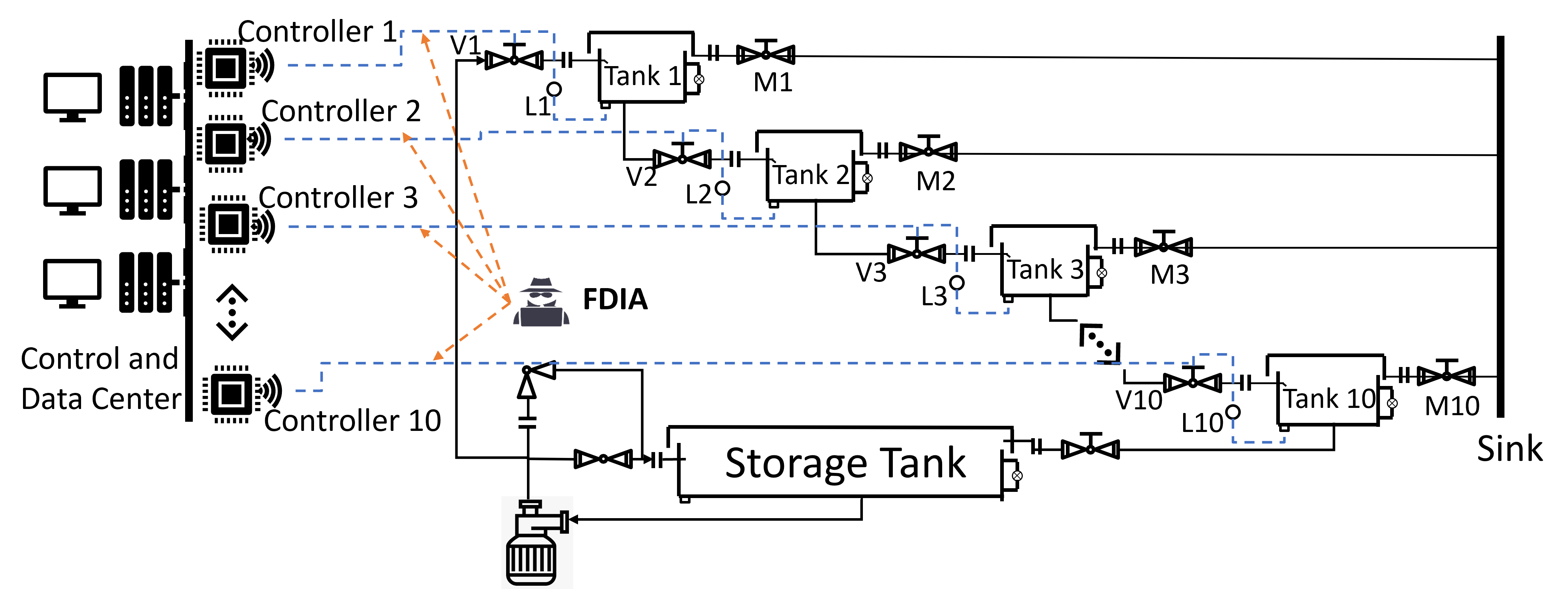This water distribution system is an 11-tanks system which contains 10 operating water tanks and a storage tank. The goal is to regulate all operating tanks' water levels around desired values. The magnetic valves V at the entrance pipelines of operating tanks are controlled to adjust the tank water levels. The magnetic valve at the entrance of the storage tank is fixed at a constant opening value. It is assumed that there are water level measurement sensors and pressure sensors in the pipelines.

The system has 10 states, 10 control inputs, and 61 measurements. The A,B,C,D matrices are saved in common_fcn folder.

If you want to generate a new system, follow the following steps:

• Run '/common_fcns/sys_generation_WDS.m": Generate a water distribution system dynamics, you can look into the code, define the measurement matrix based on your knowledge;
• Run '/common_fcns/Observability_analysis_WDS.m": Check the obsversability with respect to number of measurements; Take an example of the system (A,B,C,D) saved in common_fcn folder:
  
  This figure shows the system can maintain full observability if at least 42 measurements are remained. Thus, the 19 measurements are called redundant measurements which could be pruned.
• Run '/1_Attack_generation/Run_model_Prepare_M1M2.m': prepare discriminator matrix for attack generator.

Automated attack generation

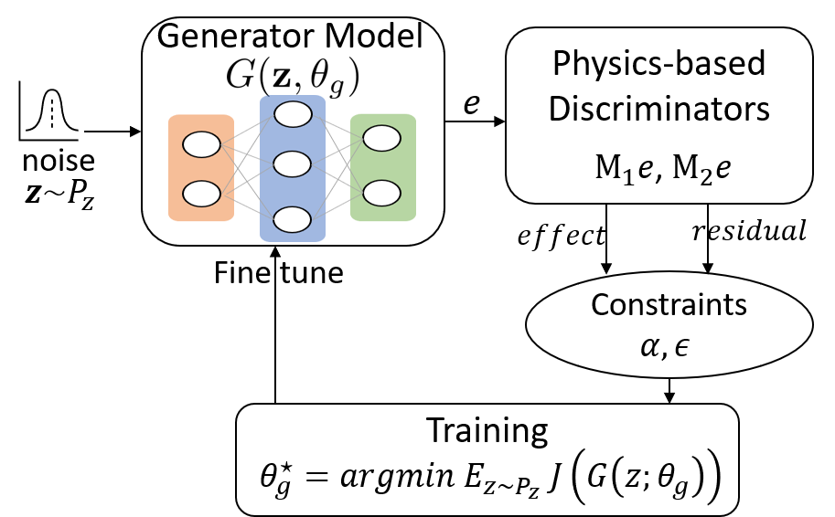
The proposed automated attack generator is an unsupervised generator trained by physics-based discriinator:

Firstly, let's do an vulnerabiliiy analysis for the system:

• Run '/1_Attack_generation/Attack_Generator_single.py': This code will generate single attack dataset corresponding to one random attack support. You can play by adjusting:

1. thresholds for effectiveness (self.tau1) line 41
2. thresholds for stelthiness (self.tau2) line 42
3. the number of attacks (n_attack) line 190

• Run '/1_Attack_generation/prepare_attack_single.m': This code pack the attack data for the preparison of testing.
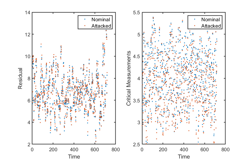
• Run '/1_Attack_generation/effect_off_attack.m': show the effect of attack in the system simulton, learn the real thrsholds corresponding to tau1, tau2.
  
  We also did some additional tests for lower frequency injection and different injection duration, the below results can be obtained

1. smaller duration
   
   This shows the duration will not affect the effect and detectability of generated attacks.
2. lower frequency
   
   This shows the atacks might be detected if they are injected to system with lower frequency. If a lower-frequency atatck wanted, we should factorize the delay in the construction of discriminator.

• Repeat the above three steps and adjust tau1, tau2 to observe a good thesholds for attack generation (untile you see a similar figrue like the above)
  Through experiment, we decide tau1= 0.1, tau2=0.5 for attack generation. And they corresponds to tau_real = 2, tau2_real =1.5 in the real system simualtion shown in the above figure.
  

Secondly, we are ready to create automated generated atatck dataset for different number of attacks and different attack support.

• Create a void folder "/1_Attack_generation/attack_dataset": make sure the folder is void
• Run '/1_Attack_generation/Attack_Generator.py': This program will take a long time, it will try to generate 5 dataset for each different number of attacks (attack support is random). For each case, it will try 40 times to train network for different attack support until the network is trained successfully. If trained successfully, an 10000 attack signal will be generated corresponding to that number of attacks and attack support. And don't worry, the dataset will be saved real time, so even if your program stop by accident, you will not lose your dataset, you could contintue program fom the stop point. A successful training will be like: (Run '/1_Attack_generation/plotting_single_attack.py')
  
• Run "/1_Attack_generation/Pack_dataset.": search all dataset under "attack dataset folder, then pack them in one cell for the convinient to use.
• Run "/1_Attack_generation/Train_dataset_gen.m": Check all generated attacks and prepare the training dataset for MLP.
• Run "/2_Training_dataset_gen/prepare_random_dataset.m": This code is to generate another random attack dataset for the fllowing comparison. Make sure you have tau_real, tau2_real in line 20,21 as you get from the vulunability analysis.

MLP training and testing

Now we have two datasets:

1. random attack dataset
2. random attack dataset + proposed automated generrated attack
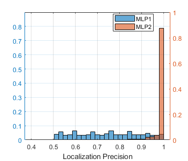
   We use dataset 1 to train an MLP1, and use dataset 2 to train an MLP2. We will show the MLP2 has better attack detection and localization performance. The detailed structure of MLPs can be found in the paper.
   

• Run '\2_MLP_training\prepare_train_dataset_for_MLP2.m': mix attack dataset to avoid one batch only contain smilar attacks.
• Run '\2_MLP_training\MLP_python.py': train MLP. change the dataset in line 22 'train_data = pd.read_csv('Dataset_for_MLP1.csv', header = None)'. After training, move the saved weights to the folder 'MLP1' or 'MLP2'.
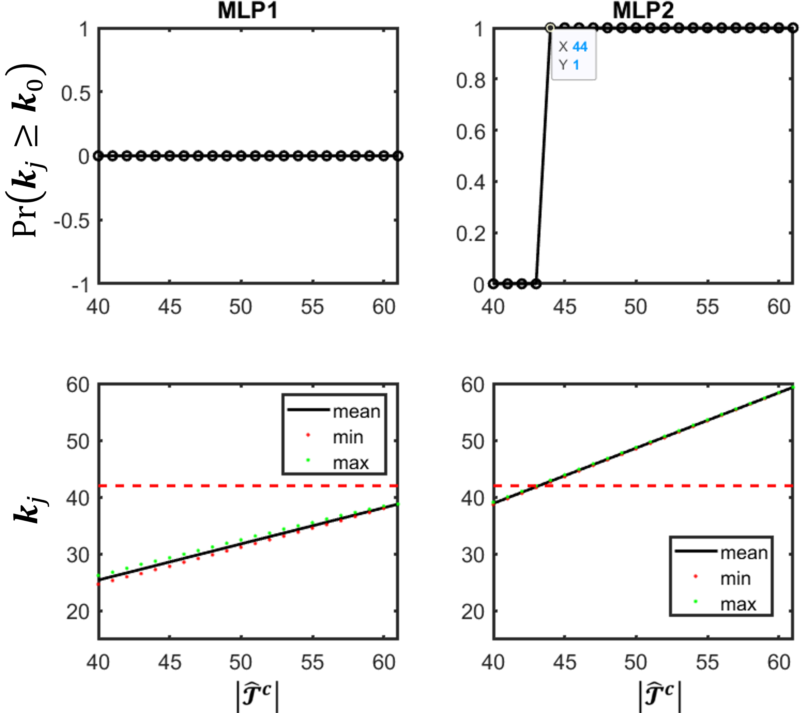
• Run '\2_MLP_training\MLP_k0.m': obtain the history accuracy of MLPs based on recivor of characterization (used in pruning algorithm later) and observe the k0 after pruning of MLPs.
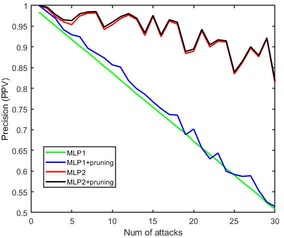
• Run '\2_MLP_training\Compare_MLPs.m': Compare the localization precision by Monte Carlo experiment
• Run '\2_MLP_training\probability_k0_bigger_than_33.m': comparison of post-pruning observability of MLPs

Concurrent learning resilient estimation - Pruning algorithm

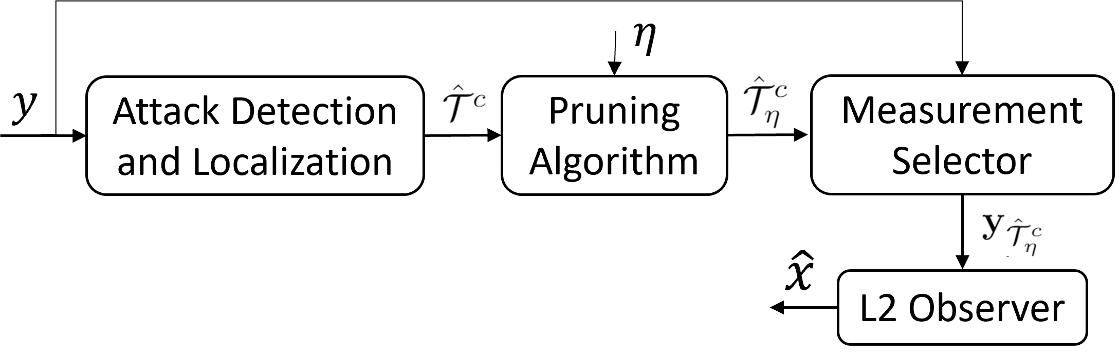
The concurrent learning-based framework is using a pruning algorithm to bridge the data-driven attack localization results and the model-based L2 estiamtor design.

• Run '\3_Sim_with_detector\Run_results_new.m': obtain all testing results
• Run '\3_Sim_with_detector\Precision_table.m': plot precision versus number of attacks
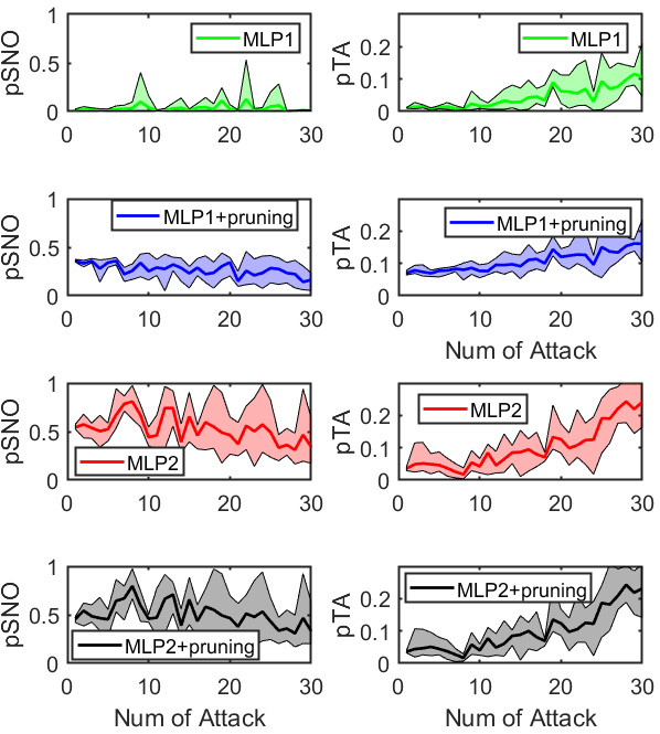
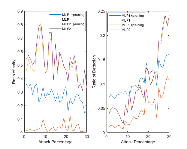
• Run '\3_Sim_with_detector\Plot_final_result.m': Plot pTA, pSNO versus number of attacks (please refer to paper for the definition of pTA and pSNO)

An example of time-domain simulation

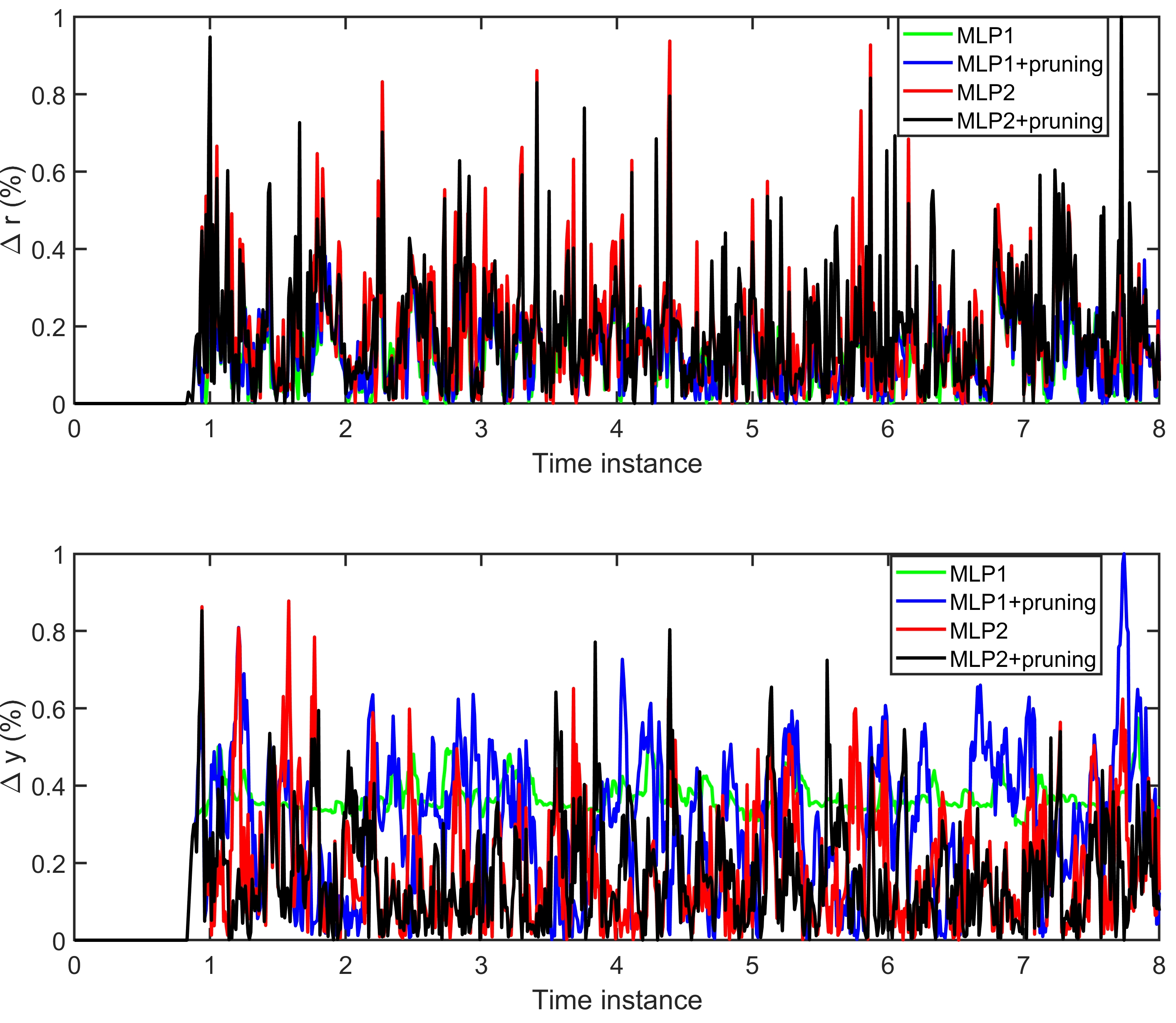
• Run '\3_Sim_with_detector\time_domian_sim.m': Run time-domain simulation, plot results