The resulting video can be found on YouTube by clicking on the image below:
The executable code can be found in: main.py
The code for the feature extraction can be found within the file feature.py.
First, all vehicle and non-vehicle images are read. For illustration an example of each class is visualized:


Then, different color spaces were explored by applying skimage.hog() which has the parameters (orientations, pixels_per_cell, and cells_per_block).
Various combinations of parameters and color spaces were tried but the final setup has been chosen as HOG features.
For the same example images as before, the YCrCb color space is used and HOG parameters of orientations=9, pixels_per_cell=(8, 8) and cells_per_block=(2, 2) are extraced. The results can be seen here:
Y Channel of Car and its HOG features:

Cr Channel of Car and its HOG features:

Cb Channel of Car and its HOG features:

Y Channel of NO Car and its HOG features:

Cr Channel of NO Car and its HOG features:

Cb Channel of NO Car and its HOG features:

Moreover, the spatial feature with spatial_size=(32,32) and histogram features with hist_bins=32 were incorporated in the final feature vector.
A linear SVM with the above mentioned feature vector and as dataset 8500 examples of each class were used. Therefore, the data set was split up in 80% training examples and 20% test examples. As a result, a test accuracy of 99.7% was achieved. The code can be find in classifier.py.
A sliding window is applied with a window size of xy_window = (96,96) and an overlap of xy_overlap = (0.5,0.5) to search for detections of cars within the bottom part of the image. Therefore, a region of interest between the y-pixel values of y_start_stop = [400,656] is applied to save runtime and only look in potential regions. This region of interest is highlighted in the following image:
![alt text][image9]
Ultimately, all detected parts of cars where gathered over the entire sliding window search. The result can be seen here.

With scipy.ndimage.measurements import label all overlapping windows are combined which leads to following final detection result.

The code can be found within heatmap.py.
For the debugging of the tracking a file debugger.py was used that saved the detection results over the project video project_video.mp4 in a JSON file. Therefore, the SVM classification only needs to be run once which speeds up the debugging of the tracking.
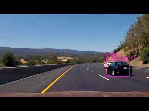
The tracking filter can be found in tracking.py and a single Track is defined in track.py. A track is simply a Bounding Box that was detection by the previous mentioned Detection step.
In each frame, the image is read from the image and first of all each existing tracks are predicted depending their stored pixel velocities with a linear motion model. Next, a data association step between the predicted tracks and the newly measured bounding boxes is performed. Therefore, a simple Nearest Neighbor Data Association is implemented that connects each track with its closest measurement if it is within a certain range. As metric, the euclidean distance of the x-coordinate, y-coordinate, width and height deviation of the compared bounding box is calculated. Whenever, this distance is below min_distance = 100 a successful association is noted. This calculation is looped over all Track-Measurement combinations and the final association is found by looking for the minimal distance.
When a track has found a measurement it is updated with a smoothing factor of scaling_measurement = 0.3 to avoid abrupt changes within the state estimation of the track. When a track has not found a measurement within the region of min_distance = 100 it is not updated but a counter not_updated is incremented. As soon as the ratio of not updated time frames falls below a threshold of threshold_bad_track = 0.85 the track is deleted. With this way, the false positive detections can be removed over time. Last but not least, when a measurement has not been assigned to a track, a new track is initialized.
The tracking result can be found in the video on the top of this page.
In the middle of the video sequence, the detection method has problems to detect the white car. A more detailed research has to be performed in future to probably adapt the feature vector or to add or change the used colorspace. Moreover, the tracking method struggles when the objects are occluded or close to each other. The occuring merging of bounding boxes or lost tracks need to be further investigated.