Because they’re just about the most important data structure there is.
Because they’re just about the most important data structure there is.
graph: collections of data represented by nodes and connections between nodes
graphs: way to formally represent network; ordered pairs
graphs: modeling relations between many items; Facebook friends (you = node; friendship = edge; bidirectional); twitter = unidirectional
graph theory: study of graphs
big O of graphs: G = V(E)
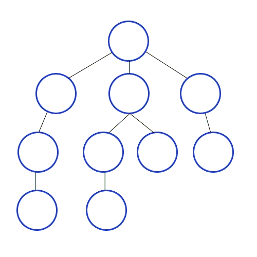
trees are a type of graph
Components required to make a graph:
- nodes or vertices: represent objects in a dataset (cities, animals, web pages)
- edges: connections between vertices; can be bidirectional
- weight: cost to travel across an edge; optional (aka cost)
Useful for:
- maps
- networks of activity
- anything you can represent as a network
- multi-way relational data
Types of Graphs:
- directed: can only move in one direction along edges; which direction indicated by arrows
- undirected: allows movement in both directions along edges; bidirectional
- cyclic: weighted; edges allow you to revisit at least 1 vertex; example weather
- acyclical: vertices can only be visited once; example recipe
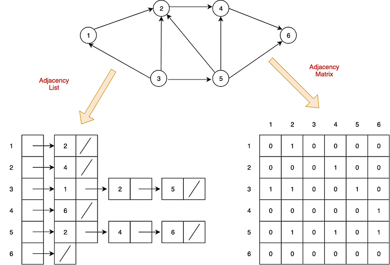
Two common ways to represent graphs in code:
- adjacency lists: graph stores list of vertices; for each vertex, it stores list of connected vertices
- adjacency matrices: two-dimensional array of lists with built-in edge weights; denotes no relationship
Both have strengths and weaknesses.
A Graph is a data structure that models objects and pairwise relationships between them with nodes and edges. For example: Users and friendships, locations and paths between them, parents and children, etc.
Graphs represent relationships between data. Anytime you can identify a relationship pattern, you can build a graph and often gain insights through a traversal. These insights can be very powerful, allowing you to find new relationships, like users who have a similar taste in music or purchasing.
Graphs can be directed or undirected, cyclic or acyclic, weighted or unweighted. They can also be represented with different underlying structures including, but not limited to, adjacency lists, adjacency matrices, object and pointers, or a custom solution.
It depends on the implementation. (Graph Representations). Before choosing an implementation, it is wise to consider the tradeoffs and complexities of the most commonly used operations.
The two most common ways to represent graphs in code are adjacency lists and adjacency matrices, each with its own strengths and weaknesses. When deciding on a graph implementation, it’s important to understand the type of data and operations you will be using.
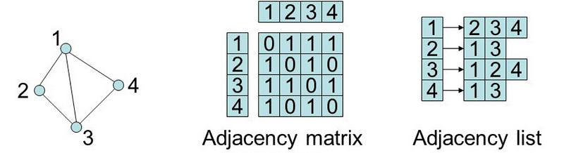
In an adjacency list, the graph stores a list of vertices and for each vertex, a list of each vertex to which it’s connected. So, for the following graph…
…an adjacency list in Python could look something like this:
class Graph:
    def __init__(self):
        self.vertices = {
                          "A": {"B"},
                          "B": {"C", "D"},
                          "C": {"E"},
                          "D": {"F", "G"},
                          "E": {"C"},
                          "F": {"C"},
                          "G": {"A", "F"}
                        }
Note that this adjacency list doesn’t actually use any lists. The vertices collection is a dictionary which lets us access each collection of edges in O(1) constant time while the edges are contained in a set which lets us check for the existence of edges in O(1) constant time.
Now, let’s see what this graph might look like as an adjacency matrix:
class Graph:
    def __init__(self):
        self.edges = [[0,1,0,0,0,0,0],
                      [0,0,1,1,0,0,0],
                      [0,0,0,0,1,0,0],
                      [0,0,0,0,0,1,1],
                      [0,0,1,0,0,0,0],
                      [0,0,1,0,0,0,0],
                      [1,0,0,0,0,1,0]]
We represent this matrix as a two-dimensional array, or a list of lists. With this implementation, we get the benefit of built-in edge weights but do not have an association between the values of our vertices and their index.
In practice, both of these would probably contain more information by including Vertex or Edge classes.
Both adjacency matrices and adjacency lists have their own strengths and weaknesses. Let’s explore their tradeoffs.
For the following:
V: Total number of vertices in the graph
E: Total number of edges in the graph
e: Average number of edges per vertex
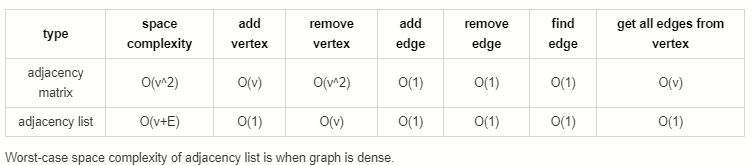
- Adjacency Matrix: O(V ^ 2)
- Adjacency List: O(V + E)
Consider a sparse graph with 100 vertices and only one edge. An adjacency list would have to store all 100 vertices but only needs to keep track of that single edge. The adjacency matrix would need to store 100x100=10,000 possible connections, even though all but one would be 0.
Now consider a dense graph where each vertex points to each other vertex. In this case, the total number of edges will approach V² so the space complexities of each are comparable. However, dictionaries and sets are less space efficient than lists so for dense graphs, the adjacency matrix is more efficient.
Takeaway: Adjacency lists are more space efficient for sparse graphs while adjacency matrices become efficient for dense graphs.
- Adjacency Matrix: O(V)
- Adjacency List: O(1)
Adding a vertex is extremely simple in an adjacency list:
self.vertices["H"] = set()
Adding a new key to a dictionary is a constant-time operation.
For an adjacency matrix, we would need to add a new value to the end of each existing row, then add a new row at the end.
for v in self.edges:
  self.edges[v].append(0)
v.append([0] * len(self.edges + 1))
Remember that with Python lists, appending to the end of a list is usually O(1) due to over-allocation of memory but can be O(n) when the over-allocated memory fills up. When this occurs, adding the vertex can be O(V²).
Takeaway: Adding vertices is very efficient in adjacency lists but very inefficient for adjacency matrices.
- Adjacency Matrix: O(V ^ 2)
- Adjacency List: O(V)
Removing vertices is pretty inefficient in both representations. In an adjacency matrix, we need to remove the removed vertex’s row, then remove that column from each other row. Removing an element from a list requires moving everything after that element over by one slot which takes an average of V/2 operations. Since we need to do that for every single row in our matrix, that results in a V² time complexity. On top of that, we need to reduce the index of each vertex after our removed index by 1 as well which doesn’t add to our quadratic time complexity, but does add extra operations.
For an adjacency list, we need to visit each vertex and remove all edges pointing to our removed vertex. Removing elements from sets and dictionaries is a O(1) operation, so this results in an overall O(V) time complexity.
Takeaway: Removing vertices is inefficient in both adjacency matrices and lists but more inefficient in matrices.
- Adjacency Matrix: O(1)
- Adjacency List: O(1)
Adding an edge in an adjacency matrix is quite simple:
self.edges[v1][v2] = 1
Adding an edge in an adjacency list is similarly simple:
self.vertices[v1].add(v2)
Both are constant-time operations.
Takeaway: Adding edges to both adjacency lists and matrices is very efficient.
- Adjacency Matrix: O(1)
- Adjacency List: O(1)
Removing an edge from an adjacency matrix is quite simple:
self.edges[v1][v2] = 0
Removing an edge from an adjacency list is similarly simple:
self.vertices[v1].remove(v2)
Both are constant-time operations.
Takeaway: Removing edges from both adjacency lists and matrices is very efficient.
- Adjacency Matrix: O(1)
- Adjacency List: O(1)
Finding an edge in an adjacency matrix is quite simple:
return self.edges[v1][v2] > 0
Finding an edge in an adjacency list is similarly simple:
return v2 in self.vertices[v1]
Both are constant-time operations.
Takeaway: Finding edges from both adjacency lists and matrices is very efficient.
- Adjacency Matrix: O(V)
- Adjacency List: O(1)
Say you want to know all the edges originating from a particular vertex. With an adjacency list, this is as simple as returning the value from the vertex dictionary:
return self.vertex[v]
In an adjacency matrix, however, it’s a bit more complicated. You would need to iterate through the entire row and populate a list based on the results:
v_edges = []
for v2 in self.edges[v]:
    if self.edges[v][v2] > 0:
        v_edges.append(v2)
return v_edges
Takeaway: Fetching all edges is more efficient in an adjacency list than an adjacency matrix.
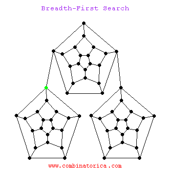
Can use breadth-first search when searching a graph; explores graph outward in rings of increasing distance from starting vertex; never attempts to explore vertex it is or has already explored
- pathfinding, routing
- web crawlers
- find neighbor nodes in P2P network
- finding people/connections away on social network
- find neighboring locations on graph
- broadcasting on a network
- cycle detection in a graph
- finding connected components
- solving several theoretical graph problems
It’s useful to color vertexes as you arrive at them and as you leave them behind as already searched.
unlisted: white
vertices whose neighbors are being explored: gray
vertices with no unexplored neighbors: black
def BFS(graph, start_vert):
    for v of graph.vertices:
        v.color = white
    start_vert.color = gray
    queue.enqueue(start_vert)
    while !queue isEmpty():
    # peek at head but don't dequeue
    u = queue[0]
    for v of u.neighbors:
        if v.color == white:
            v.color == gray
            queue.enqueue(v)
    queue.dequeue()
    u.color = black
- Mark graph vertices white.
- Mark starting vertex gray.
- Enqueue starting vertex.
- Check if queue is not empty.
- If not empty, peek at first item in queue.
- Loop through that vertex’s neighbors.
- Check if unvisited.
- If unvisited, mark as gray and enqueue vertex.
- Dequeue current vertex and mark as black.
- Repeat until all vertices are explored.
dives down the graph as far as it can before backtracking and exploring another branch; never attempts to explore a vertex it has already explored or is in the process of exploring; exact order will vary depending on which branches get taken first and which is starting vertex
- preferred method for exploring a graph if we want to ensure we visit every node in graph
- finding minimum spanning trees of weighted graphs
- pathfinding
- detecting cycles in graphs
- solving and generating mazes
- topological sorting, useful for scheduling sequences of dependent jobs
# recursion
def explore(graph):
    visit(this_vert)
    explore(remaining_graph)

# iterative
def DFS(graph):
    for v of graph.verts:
        v.color = white
        v.parent = null
    for v of graph.verts:
        if v.color == white:
            DFS_visit(v)

def DFS_visit(v):
    v.color = gray
    for neighbor of v.adjacent_nodes:
        if neighbor.color == white:
            neighbor.parent = v
            DFS_visit(neighbor)
    v.color = black
- Take graph as parameter.
- Marks all vertices as unvisited.
- Sets vertex parent as null.
- Passes each unvisited vertex into DFS_visit().
- Mark current vertex as gray.
- Loops through its unvisited neighbors.
- Sets parent and makes recursive call to DFS_visit().
- Marks vertex as black.
- Repeat until done.
connected components: in a disjoint graph, groups of nodes on a graph that are connected with each other
- typically very large graphs, networks
- social networks
- networks (which devices can reach one another)
- epidemics (how spread, who started, where next)
key to finding connected components: searching algorithms, breadth-first search
- for each node in graph:
- has it been explored
- if no, do BFS
- all nodes reached are connected
- if yes, already in connected component
- go to next node
strongly connected components: any node in this group can get to any other node
'''

This Bellman-Ford Code is for determination whether we can get

shortest path from given graph or not for single-source shortest-paths problem.

In other words, if given graph has any negative-weight cycle that is reachable

from the source, then it will give answer False for "no solution exits".

For argument graph, it should be a dictionary type

such as

graph = {

'a': {'b': 6, 'e': 7},

'b': {'c': 5, 'd': -4, 'e': 8},

'c': {'b': -2},

'd': {'a': 2, 'c': 7},

'e': {'b': -3}

}

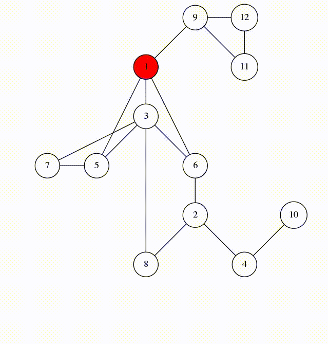
- A graph is any collection of nodes and edges.
- A graph is a less restrictive class of collections of nodes than structures like a tree.
- It doesn’t need to have a root node (not every node needs to be accessible from a single node)
- It can have cycles (a group of nodes whose paths begin and end at the same node)
Undirected Graph: An undirected graph is one where the edges do not specify a particular direction. The edges are bi-directional.
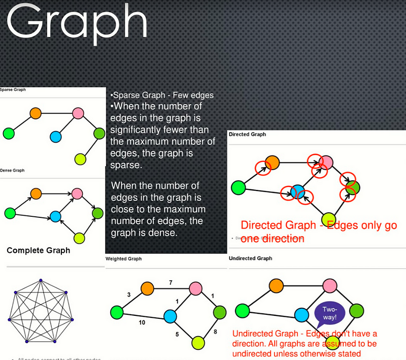
- Dense Graph — A graph with lots of edges.
- “Dense graphs have many edges. But, wait!
⚠️ I know what you must be thinking, how can you determine what qualifies as “many edges”? This is a little bit too subjective, right? ? I agree with you, so let’s quantify it a little bit: - Let’s find the maximum number of edges in a directed graph. If there are |V| nodes in a directed graph (in the example below, six nodes), that means that each node can have up to |v| connections (in the example below, six connections).
- Why? Because each node could potentially connect with all other nodes and with itself (see “loop” below). Therefore, the maximum number of edges that the graph can have is |V|\*|V| , which is the total number of nodes multiplied by the maximum number of connections that each node can have.”
- When the number of edges in the graph is close to the maximum number of edges, the graph is dense.
- Sparse Graph — Few edges
- When the number of edges in the graph is significantly fewer than the maximum number of edges, the graph is sparse.
- Weighted Graph — Edges have a cost or a weight to traversal
- Directed Graph — Edges only go one direction
- Undirected Graph — Edges don’t have a direction. All graphs are assumed to be undirected unless otherwise stated
Uses a class to define the neighbors as properties of each node.
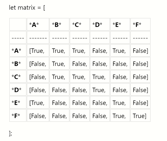
The row index will correspond to the source of an edge and the column index will correspond to the edges destination.
- When the edges have a direction,
matrix[i][j]may not be the same asmatrix[j][i] - It is common to say that a node is adjacent to itself so
matrix[x][x]is true for any node - Will be O(n²) space complexity
Seeks to solve the shortcomings of the matrix implementation. It uses an object where keys represent node labels and values associated with that key are the adjacent node keys held in an array.
By Bryan Guner on June 3, 2021.
Exported from Medium on August 6, 2021.