README.md

GrowthMaps

GrowthMaps.jl produces gridded population level growth rates from environmental data, and fitted growth and stress models, following the method outlined in Maino et al, "Forecasting the potential distribution of the invasive vegetable leafminer using ‘top-down’ and ‘bottom-up’ models" (in press).

GrowthMaps.jl is an alternative to CLIMEX and similar tools. Its key point of differentiation from other methods is that results arrays have units of growth/time. Another useful property of these models is that growth rate layers can be added and combined arbitrarily.

A primary use-case for GrowthMaps layers is in for calculating growth-rates for . This allows heterogeneous organism growth rates to influence dispersal patterns, simulating permanent range limits and potential for seasonal range shift.

For data input, this package leverages GeoData.jl to import datasets from many different sources. Files are loaded lazily in sequence to minimise memory, using the GeoSeries abstraction, that can hold "SMAP" HDF5 files, NetCDFs, or GeoStacks of tif or other GDAL source files, or simply memory-backed arrays. These data sources can be used interchangeably.

Computations can be run on GPUs, for example with arraytype=CuArray to use CUDA for Nvidia GPUs.

Example

Here we run a single growth model over SMAP data, on a Nvida GPU:

using GrowthMaps, GeoData, HDF5, CUDA, Unitful

# Define a growth model
p = 3e-01
ΔH_A = 3e4cal/mol
ΔH_L = -1e5cal/mol
ΔH_H = 3e5cal/mol
Thalf_L = 2e2K
Thalf_H = 3e2K
T_ref = K(25.0°C)
growthmodel = SchoolfieldIntrinsicGrowth(p, ΔH_A, ΔH_L, Thalf_L, ΔH_H, Thalf_H, T_ref)

# Wrap the model with a data layer with the key
# to retreive the data from, and the Unitful.jl units.
growth = Layer(:surface_temp, K, growthmodel)

Now we will use GeoData.jl to load a series of SMAP files lazily, and GrowthMaps.jl will load them to the GPU just in time for processing:

# Load 1000s of HDF5 files lazily using GeoData.jl
series = SMAPseries("your_SMAP_folder")

# Run the model
output = mapgrowth(growth;
    series=series,
    tspan=DateTime(2016, 1):Month(1):DateTime(2016, 12),
    arraytype=CuArray, # Use an Nvidia GPU for computations
)

# Plot every third month of 2016:
output[Ti(1:3:12)] |> plot

GrowthMaps.jl is fast.

As a rough benchmark, running a model using 3 3800*1600 layers from 3000 SMAP files on a M.2. drive takes under 7 minutes on a desktop with a good GPU, like a GeForce 1080. The computation time is trivial, running ten similar models takes essentially the same time as running one model. On a CPU, model run-time becomes more of a factor, but is still fast for a single model.

See the Examples section in the documentation to get started. You can also work through the example.jmd in atom (with the language-weave plugin) or the notebook.

Live Interfaces

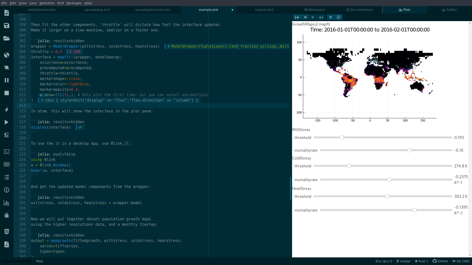
GrowthMaps provides interfaces for manually fitting models where automated fits are not appropriate.

Model curves can be fitted to an AbstractRange of input data using manualfit:

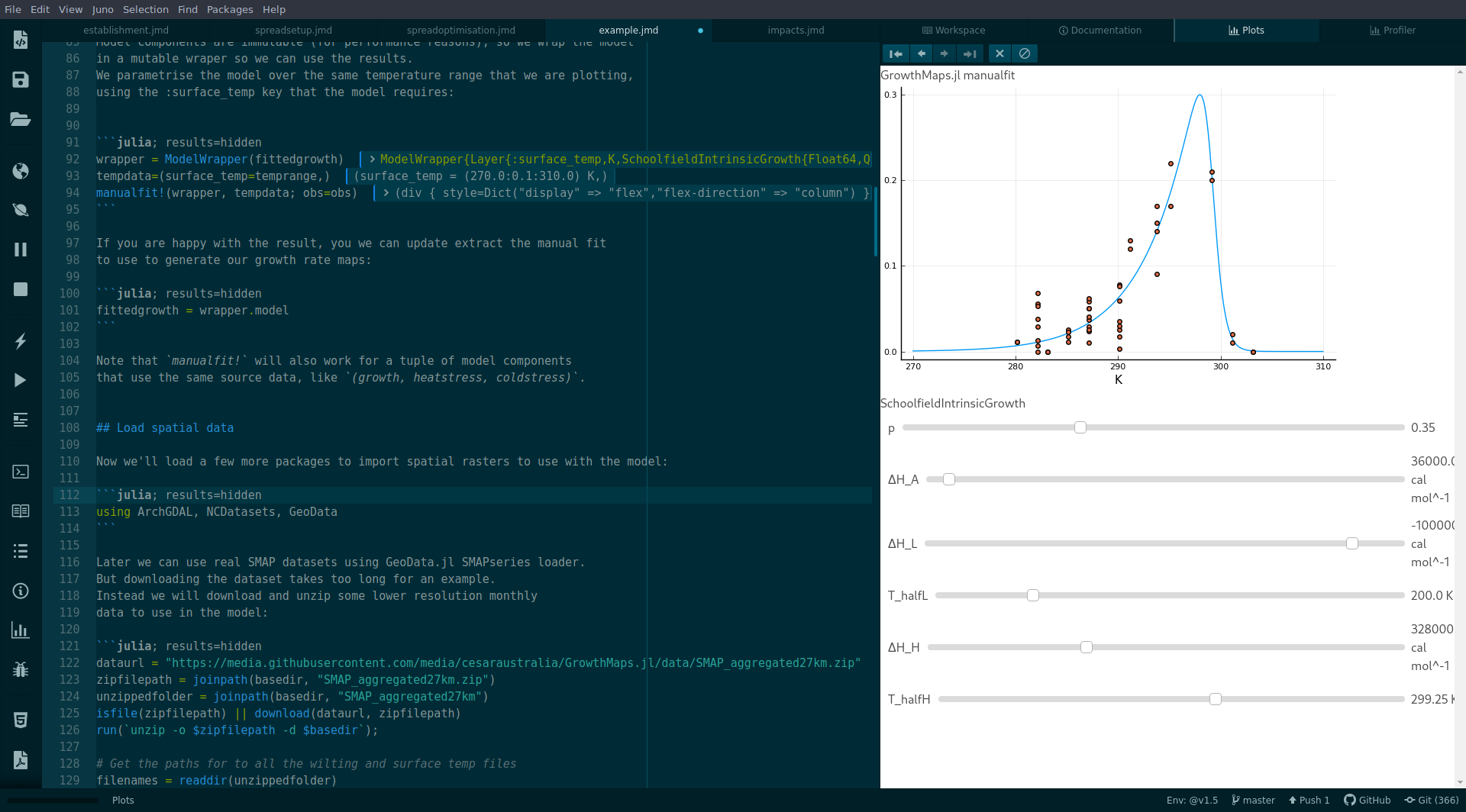
Observations can be fitted to a map. Aggregated maps GeoSeries can be used to fit models in real-time. See the examples for details.