Advanced Lane Finding

This My test video

In this project, my goal is to write a software pipeline to identify the lane boundaries in a video.

Overview

---

When we drive, we use our eyes to decide where to go. The lines on the road that show us where the lanes are act as our constant reference for where to steer the vehicle. Naturally, one of the first things we would like to do in developing a self-driving car is to automatically detect lane lines using an algorithm.

The Project

The goals / steps of this project are the following:

• Camera Calibration
• Apply a distortion correction to raw images.
• Use color transforms, gradients, etc., to create a thresholded binary image.
• Apply a perspective transform to rectify binary image ("birds-eye view").
• Detect lane pixels and fit to find the lane boundary.
• Determine the curvature of the lane and vehicle position with respect to center.
• Warp the detected lane boundaries back onto the original image.
• Output visual display of the lane boundaries and numerical estimation of lane curvature and vehicle position.

My pipeline consisted of some steps.

• 01.Compute the camera calibration matrix and distortion coefficients given a set of chessboard images.
• 02.Apply a distortion correction to raw images.
• 03.Use color transforms, gradients, etc., to create a thresholded binary image.
• 04.Use to correctly rectify each image to a "birds-eye view"
• 05.Identified lane-line pixels and fit their positions
• 06.Determine the curvature of the lane and vehicle position with respect to center
• 07.Warp the detected lane boundaries back onto the original image.
• 08.Pipeline_video

01.Compute the camera calibration matrix and distortion coefficients given a set of chessboard images.

In this stage, I read in some test images and processed the camera corrections according to the way the course taught. However, some images were found to be unrecognizable during the calibration process, so the Internet searched for relevant data and found that the input image did not necessarily match the desired image. So I tried to fine-tune Nx, Ny up and down, still can't read two pictures. So I chose to exclude two images and use other images as the correction pattern.

#Tried to fine-tune Nx, Ny up and down
if ('calibration1.jpg' in image_name):
    nx = 9
    ny = 5
else:
    nx = 9
    ny = 6

Result

02.Apply a distortion correction to raw images.

After camera correction, I saved the parameters in PKL form. The parameters are then referenced in this stage and applied to each image.

import pickle

f = open('Camera_parameters.pkl', 'wb')
pickle.dump(mtx, f)
pickle.dump(dist, f)
f.close()

Result

03.Use color transforms, gradients, etc., to create a thresholded binary image.

In this stage,I tried to use the various color leathers I found in the documentation to transform the image and find a workable solution in it.

for image_name in os.listdir("output_images/Undistorted_Image/"):
    #read in each image
    image = mpimg.imread("output_images/Undistorted_Image/" + image_name)
    #Show Color
    fig, axs = plt.subplots(4,3, figsize=(20, 20))
    axs = axs.ravel()

    axs[0].imshow(image[:,:,0], cmap='gray')
    axs[0].set_title('R-channel', fontsize=30)
    axs[1].imshow(image[:,:,1], cmap='gray')
    axs[1].set_title('G-Channel', fontsize=30)
    axs[2].imshow(image[:,:,2], cmap='gray')
    axs[2].set_title('B-channel', fontsize=30)

    image_HSV = cv2.cvtColor(image, cv2.COLOR_RGB2HSV)
    axs[3].imshow(image_HSV[:,:,0], cmap='gray')
    axs[3].set_title('H-Channel', fontsize=30)
    axs[4].imshow(image_HSV[:,:,1], cmap='gray')
    axs[4].set_title('S-channel', fontsize=30)
    axs[5].imshow(image_HSV[:,:,2], cmap='gray')
    axs[5].set_title('V-Channel', fontsize=30)

    image_HLS = cv2.cvtColor(image, cv2.COLOR_RGB2HLS)
    axs[6].imshow(image_HLS[:,:,0], cmap='gray')
    axs[6].set_title('H-Channel', fontsize=30)
    axs[7].imshow(image_HLS[:,:,1], cmap='gray')
    axs[7].set_title('L-channel', fontsize=30)
    axs[8].imshow(image_HLS[:,:,2], cmap='gray')
    axs[8].set_title('S-Channel', fontsize=30)
    
    image_LAB = cv2.cvtColor(image, cv2.COLOR_RGB2LAB)
    axs[9].imshow(image_LAB[:,:,0], cmap='gray')
    axs[9].set_title('L-Channel', fontsize=30)
    axs[10].imshow(image_LAB[:,:,1], cmap='gray')
    axs[10].set_title('A-channel', fontsize=30)
    axs[11].imshow(image_LAB[:,:,2], cmap='gray')
    axs[11].set_title('B-Channel', fontsize=30)

Result

After finding the color, I try to find the upper and lower thresholds as filters.

Define function

def HLS_S_threshold(img, threshold=(200, 255)):

    HLS_img = cv2.cvtColor(img, cv2.COLOR_RGB2HLS)
    
    HLS_S_img = HLS_img[:,:,2]
    
    HLS_S_img = HLS_S_img*(255/np.max(HLS_S_img))
    
    binary_output = np.zeros_like(HLS_S_img)
    
    binary_output[(HLS_S_img > threshold[0]) & (HLS_S_img <= threshold[1])] = 1

    return binary_output

Show Result

for image_name in os.listdir("output_images/Undistorted_Image/"):
    #read in each image
    image = mpimg.imread("output_images/Undistorted_Image/" + image_name)
    
    #It is best to test the threshold of that section.
    #Show Result
    fig, axs = plt.subplots(1,3, figsize=(20, 9))
    axs = axs.ravel()
    axs[0].imshow(HLS_S_threshold(image, threshold=(0, 80)))
    axs[0].set_title('HLS_S-0-80-Channel', fontsize=30)
    axs[1].imshow(HLS_S_threshold(image, threshold=(80, 160)))
    axs[1].set_title('HLS_S-80-160-Channel', fontsize=30)
    axs[2].imshow(HLS_S_threshold(image, threshold=(160, 255)))
    axs[2].set_title('HLS_S-160-255-Channel', fontsize=30)
    
    

Result

After testing, you can know that 160 is the most suitable.

Next, apply sobel and find the upper and lower thresholds.

Finally, combined with the two to get a color pattern, we can easily identify the two different channels combined image.

04.Use to correctly rectify each image to a "birds-eye view"

To convert to a birds-eye view, first mark the places that need to be turned into a birds-eye view. We take the trapezoid of the road position, just like P1.

def unwarp(img):
    image_size = (img.shape[1], img.shape[0])
    src = np.float32([(585,460),
                  (700,460), 
                  (260,680), 
                  (1000,680)])

    dst = np.float32([(300,0),
                      (image_size[0]-300,0),
                      (300,image_size[1]),
                      (image_size[0]-300,image_size[1])])
    img_size = (img.shape[1], img.shape[0])
    # use cv2.getPerspectiveTransform() to get M, the transform matrix, and Minv, the inverse
    M = cv2.getPerspectiveTransform(src, dst)
    
    Minv = cv2.getPerspectiveTransform(dst, src)
    
    # Warp the image using OpenCV warpPerspective()
    warped = cv2.warpPerspective(img, M, img_size, flags=cv2.INTER_LINEAR)
    
    return warped, M, Minv

Result

05.Identified lane-line pixels and fit their positions

First, we combine the two images Combined and Birds_Eye_View

Then we use the Np.hstack function learned in the course to find the position of the line. And use the Slide Window to continuously search the entire image.

# Identify the x and y positions of all nonzero pixels in the image
    nonzero = binary_warped.nonzero()
    nonzeroy = np.array(nonzero[0])
    nonzerox = np.array(nonzero[1])
    
    # Current positions to be updated later for each window in nwindows
    leftx_current = leftx_base
    rightx_current = rightx_base

    # Create empty lists to receive left and right lane pixel indices
    left_lane_inds = []
    right_lane_inds = []

    # Step through the windows one by one
    for window in range(nwindows):
        # Identify window boundaries in x and y (and right and left)
        win_y_low = binary_warped.shape[0] - (window+1)*window_height
        win_y_high = binary_warped.shape[0] - window*window_height
        win_xleft_low = leftx_current - margin
        win_xleft_high = leftx_current + margin
        win_xright_low = rightx_current - margin
        win_xright_high = rightx_current + margin
        
        # Draw the windows on the visualization image
        cv2.rectangle(out_img,(win_xleft_low,win_y_low),
        (win_xleft_high,win_y_high),(0,255,0), 2) 
        cv2.rectangle(out_img,(win_xright_low,win_y_low),
        (win_xright_high,win_y_high),(0,255,0), 2) 
        
        # Identify the nonzero pixels in x and y within the window #
        good_left_inds = ((nonzeroy >= win_y_low) & (nonzeroy < win_y_high) & 
        (nonzerox >= win_xleft_low) &  (nonzerox < win_xleft_high)).nonzero()[0]
        good_right_inds = ((nonzeroy >= win_y_low) & (nonzeroy < win_y_high) & 
        (nonzerox >= win_xright_low) &  (nonzerox < win_xright_high)).nonzero()[0]
        
        # Append these indices to the lists
        left_lane_inds.append(good_left_inds)
        right_lane_inds.append(good_right_inds)
        
        # If you found > minpix pixels, recenter next window on their mean position
        if len(good_left_inds) > minpix:
            leftx_current = np.int(np.mean(nonzerox[good_left_inds]))
        if len(good_right_inds) > minpix:        
            rightx_current = np.int(np.mean(nonzerox[good_right_inds]))

Result

Then according to the polynomial obtained by Slide Windows, do the approximate search in the following pictures.

        # Identify the nonzero pixels in x and y within the window #
        good_left_inds = ((nonzeroy >= win_y_low) & (nonzeroy < win_y_high) & 
        (nonzerox >= win_xleft_low) &  (nonzerox < win_xleft_high)).nonzero()[0]
        good_right_inds = ((nonzeroy >= win_y_low) & (nonzeroy < win_y_high) & 
        (nonzerox >= win_xright_low) &  (nonzerox < win_xright_high)).nonzero()[0]

inplace

    left_lane_inds = ((nonzerox > (left_fit[0]*(nonzeroy**2) + left_fit[1]*nonzeroy + 
                    left_fit[2] - margin)) &\
                    (nonzerox < (left_fit[0]*(nonzeroy**2) + 
                    left_fit[1]*nonzeroy + left_fit[2] + margin)))
    right_lane_inds = ((nonzerox > (right_fit[0]*(nonzeroy**2) + right_fit[1]*nonzeroy + 
                    right_fit[2] - margin)) &\
                    (nonzerox < (right_fit[0]*(nonzeroy**2) + 
                    right_fit[1]*nonzeroy + right_fit[2] + margin)))

06.Determine the curvature of the lane and vehicle position with respect to center

Because Project assumes that the center of the picture is the center point, we only need to divide the width of the picture by 2 to be the center point of the car. The center point of the lane can be obtained by taking the center point from the curve obtained from the polynomial.

def measure_curvature_pixels_in_realworld(ploty, leftx, lefty, rightx, righty, left_fit, right_fit):
    # meters per pixel in y dimension
    ym_per_pix = 30/720 
    # meters per pixel in x dimension
    xm_per_pix = 3.7/720
    # Reverse to match top-to-bottom in y
    leftx = leftx[::-1]  
    # Reverse to match top-to-bottom in y
    rightx = rightx[::-1]  
    # Define y-value where we want radius of curvature
    # We'll choose the maximum y-value, corresponding to the bottom of the image
    y_eval = np.max(ploty)

    left_lane = np.mean(left_fit[0]*y_eval**2 + left_fit[1]*y_eval + left_fit[2])

    right_lane = np.mean(right_fit[0]*y_eval**2 + right_fit[1]*y_eval + right_fit[2])

    car_position = combined_binary.shape[1]/2

    center_lane_point = (left_lane + right_lane) /2

    center_miss = (car_position - center_lane_point) * xm_per_pix

    left_fit_cr = np.polyfit(lefty*ym_per_pix, leftx*xm_per_pix, 2)

    right_fit_cr = np.polyfit(righty*ym_per_pix, rightx*xm_per_pix, 2)

    
    
    # Calculation of R_curve (radius of curvature)
    left_curverad = ((1 + (2*left_fit_cr[0]*y_eval*ym_per_pix + left_fit_cr[1])**2)**1.5) / np.absolute(2*left_fit_cr[0])
    right_curverad = ((1 + (2*right_fit_cr[0]*y_eval*ym_per_pix + right_fit_cr[1])**2)**1.5) / np.absolute(2*right_fit_cr[0])
    
    return left_curverad, right_curverad, center_miss

07.Warp the detected lane boundaries back onto the original image.

At this stage, I first read in the image, then made a capture of the location of the lane and converted it to a binary image.

#read in each image
original_image = mpimg.imread("test_images/" + image_name)

undistort_image = undistort(original_image)

unwarp_image, M, Minv = unwarp(undistort_image)

#Applies a Gaussian Noise kernel
blur_image = gaussian_blur(unwarp_image, kernel_size=7)

binary_image1 = abs_sobel_thresh(blur_image,orient='x',thresh=(60, 255))

binary_image2 = HLS_S_threshold(blur_image, threshold=(160, 190))

combined_binary = combine_binary(binary_image1, binary_image2)

Then based on the binary picture, find the polynomial of the lane line.

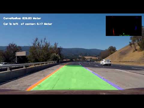
curverad, center_miss, left_fit, right_fit= fit_polynomial(combined_binary)

Then draw the polynomial of the left and right lanes into red and blue lines, and fill the green squares in the middle of the line. Continue to find the actual distance and paste the distance onto the picture.

def info_image(original_img, combined_binary, left_fit, right_fit, Minv, curverad, center_miss):

    ploty = np.linspace(0, combined_binary.shape[0]-1, combined_binary.shape[0])
    
    left_fitx = left_fit[0]*ploty**2 + left_fit[1]*ploty + left_fit[2]
    right_fitx = right_fit[0]*ploty**2 + right_fit[1]*ploty + right_fit[2]

    new_image = np.copy(original_img)

    window_img = np.zeros((combined_binary.shape[0],combined_binary.shape[1],3), np.uint8)

    left_line_pts = np.array([np.transpose(np.vstack([left_fitx, ploty]))])

    right_line_pts = np.array([np.flipud(np.transpose(np.vstack([right_fitx, ploty])))])

    line_pts = np.hstack((left_line_pts, right_line_pts))

    cv2.fillPoly(window_img, np.int_([line_pts]), (0,255, 0))
    cv2.polylines(window_img, np.int32([left_line_pts]), color=(255,0,0), thickness=50, isClosed=False)
    cv2.polylines(window_img, np.int32([right_line_pts]), color=(0,0,255), thickness=50, isClosed=False)

    diswarp_lane_image = cv2.warpPerspective(window_img, Minv, (combined_binary.shape[1], combined_binary.shape[0]))

    # Combine the result with the original image
    result = cv2.addWeighted(new_image, 1, diswarp_lane_image, 0.3, 0)

    font = cv2.FONT_HERSHEY_PLAIN
    text= "CurveRadius: " + "{:03.2f}".format(curverad) + " Meter"

    cv2.putText(result, text, (30,50), font, 1.5, (255,255,255), 3, cv2.LINE_AA)

    message = ''
    if center_miss > 0:
        text = "Car is right of center: " "{:03.2f}".format(center_miss) + " Meter" 
    elif center_miss < 0:
        text = "Car is left  of center: " "{:03.2f}".format(abs(center_miss)) + " Meter" 

    cv2.putText(result, text, (30,100), font, 1.5, (255,255,255), 3, cv2.LINE_AA)
    
    return result

Result

08.Pipeline_video

In summary, we are going to start video streaming. Because video has the problem of light and shadow changes, sometimes the lane line will not be found.

def process_image(original_image):    
    global left_fit_prev
    global right_fit_prev
    global curverad_prev
    global center_miss_prev
    # HYPERPARAMETER
    global margin

So I directly do a global variable to get the information of the previous picture, because we can assume that the lane line is a continuously changing polynomial.

Then I did some pre-processing on the image. For the lower noise, I used cv2.bilateralFilter once, but the processing efficiency and the effect were not good, so I still used the original way to deal with it.

    alpha = 0.001

    undistort_image = undistort(original_image)
    
    unwarp_image, M, Minv = unwarp(undistort_image)

    blur_image = gaussian_blur(unwarp_image, kernel_size=7)
    
    binary_image1 = abs_sobel_thresh(blur_image,orient='x',thresh=(60, 255))
    
    binary_image2 = HLS_S_threshold(blur_image, threshold=(160, 190))
    
    combined_binary = combine_binary(binary_image1, binary_image2)

The following judgment logic is as follows:

1. If it is the first picture, use slide windows.

    if (left_fit_prev is None):
        margin = 100
        curverad, center_miss, left_fit, right_fit= fit_polynomial(combined_binary)
        curverad_prev = curverad
        center_miss_prev = center_miss
        left_fit_prev = left_fit
        right_fit_prev = right_fit

2. If no lane line is detected (may be due to noise such as light and shadow), use the parameters of the previous picture.

    else:
        curverad, center_miss, left_fit, right_fit= search_around_poly(combined_binary, left_fit_prev, right_fit_prev)
        if (left_fit is None or right_fit is None):
            curverad = curverad_prev
            center_miss = center_miss_prev
            left_fit = left_fit_prev
            right_fit = right_fit_prev
        else:

3. If one of the lane lines changes too much, the polynomial of the other lane is applied with the first coefficient and the second coefficient (we can assume that the lane is parallel and wide) because the third is the lane position.

            if abs((abs(right_fit[0]-right_fit_prev[0])*10**5) - (abs(left_fit[0]-left_fit_prev[0])*10**5)) > 30:
                if abs(right_fit[0]-right_fit_prev[0])*10**5 > abs(left_fit[0]-left_fit_prev[0])*10**5:
                    right_fit[0] = left_fit_prev[0]
                    right_fit[1] = left_fit_prev[1]
                    right_fit[2] = right_fit_prev[2]
                else:
                    left_fit[0] = right_fit_prev[0]
                    left_fit[1] = right_fit_prev[1]
                    left_fit[2] = left_fit_prev[2]
                margin = 100
                curverad = curverad_prev
                center_miss = center_miss_prev
                #left_fit = left_fit_prev
                #right_fit = right_fit_prev
            else:
                margin = 100
                curverad_prev = curverad
                center_miss_prev = center_miss
                left_fit_prev = left_fit
                right_fit_prev = right_fit

4. Finally, to prevent excessive noise, I set an alpha to weight the polynomial coefficients of the previous frame and the coefficients of this image.

        left_fit = left_fit*alpha + left_fit_prev*(1-alpha)
        right_fit = right_fit*alpha + right_fit_prev*(1-alpha)
        
        

    drawed_image = info_image(original_image, combined_binary, left_fit, right_fit, Minv,curverad, center_miss)
    return drawed_image

Discussion

Briefly discuss any problems / issues you faced in your implementation of this project. Where will your pipeline likely fail? What could you do to make it more robust?

I tried to do the processing on the challenge video, which obviously failed. I think it is because of the lane line identification and the problem of noise processing. In addition, the quadrilateral frame I set cannot be processed on the mountain road video, and should be wider. I think the way to improve can be handled with continuous polynomials, because the lanes are all parallel, and I can boldly assume that the car will be around the center of the lane. We can know that the intercept of the polynomial should have an average. We can find a lot of polynomials, and then take two lines with the closest two coefficients and one lane wide as the lane line. This can eliminate noise very well. Another attempt is to make a mask for the lane center and periphery of the previous frame when the image is preprocessed, and then search for the lane line for the inside, which is more efficient than direct search. .

After first Review

After the first submission review, I found a bug in my program. I fixed the bug and took the inspector's suggestion to add a binary image to the image. This will understand what the computer actually saw during the operation.

Thank you for reading