/
README.md
755 lines (564 loc) · 31.1 KB
/
README.md
1
2
3
4
5
6
7
8
9
10
11
12
13
14
15
16
17
18
19
20
21
22
23
24
25
26
27
28
29
30
31
32
33
34
35
36
37
38
39
40
41
42
43
44
45
46
47
48
49
50
51
52
53
54
55
56
57
58
59
60
61
62
63
64
65
66
67
68
69
70
71
72
73
74
75
76
77
78
79
80
81
82
83
84
85
86
87
88
89
90
91
92
93
94
95
96
97
98
99
100
101
102
103
104
105
106
107
108
109
110
111
112
113
114
115
116
117
118
119
120
121
122
123
124
125
126
127
128
129
130
131
132
133
134
135
136
137
138
139
140
141
142
143
144
145
146
147
148
149
150
151
152
153
154
155
156
157
158
159
160
161
162
163
164
165
166
167
168
169
170
171
172
173
174
175
176
177
178
179
180
181
182
183
184
185
186
187
188
189
190
191
192
193
194
195
196
197
198
199
200
201
202
203
204
205
206
207
208
209
210
211
212
213
214
215
216
217
218
219
220
221
222
223
224
225
226
227
228
229
230
231
232
233
234
235
236
237
238
239
240
241
242
243
244
245
246
247
248
249
250
251
252
253
254
255
256
257
258
259
260
261
262
263
264
265
266
267
268
269
270
271
272
273
274
275
276
277
278
279
280
281
282
283
284
285
286
287
288
289
290
291
292
293
294
295
296
297
298
299
300
301
302
303
304
305
306
307
308
309
310
311
312
313
314
315
316
317
318
319
320
321
322
323
324
325
326
327
328
329
330
331
332
333
334
335
336
337
338
339
340
341
342
343
344
345
346
347
348
349
350
351
352
353
354
355
356
357
358
359
360
361
362
363
364
365
366
367
368
369
370
371
372
373
374
375
376
377
378
379
380
381
382
383
384
385
386
387
388
389
390
391
392
393
394
395
396
397
398
399
400
401
402
403
404
405
406
407
408
409
410
411
412
413
414
415
416
417
418
419
420
421
422
423
424
425
426
427
428
429
430
431
432
433
434
435
436
437
438
439
440
441
442
443
444
445
446
447
448
449
450
451
452
453
454
455
456
457
458
459
460
461
462
463
464
465
466
467
468
469
470
471
472
473
474
475
476
477
478
479
480
481
482
483
484
485
486
487
488
489
490
491
492
493
494
495
496
497
498
499
500
501
502
503
504
505
506
507
508
509
510
511
512
513
514
515
516
517
518
519
520
521
522
523
524
525
526
527
528
529
530
531
532
533
534
535
536
537
538
539
540
541
542
543
544
545
546
547
548
549
550
551
552
553
554
555
556
557
558
559
560
561
562
563
564
565
566
567
568
569
570
571
572
573
574
575
576
577
578
579
580
581
582
583
584
585
586
587
588
589
590
591
592
593
594
595
596
597
598
599
600
601
602
603
604
605
606
607
608
609
610
611
612
613
614
615
616
617
618
619
620
621
622
623
624
625
626
627
628
629
630
631
632
633
634
635
636
637
638
639
640
641
642
643
644
645
646
647
648
649
650
651
652
653
654
655
656
657
658
659
660
661
662
663
664
665
666
667
668
669
670
671
672
673
674
675
676
677
678
679
680
681
682
683
684
685
686
687
688
689
690
691
692
693
694
695
696
697
698
699
700
701
702
703
704
705
706
707
708
709
710
711
712
713
714
715
716
717
718
719
720
721
722
723
724
725
726
727
728
729
730
731
732
733
734
735
736
737
738
739
740
741
742
743
744
745
746
747
748
749
750
751
752
753
754
755
# Geomandel
[](https://travis-ci.org/crapp/geomandel)
[](#license)
[](https://github.com/crapp/geomandel/releases/latest)
<!-- START doctoc generated TOC please keep comment here to allow auto update -->
<!-- DON'T EDIT THIS SECTION, INSTEAD RE-RUN doctoc TO UPDATE -->
- [Introduction](#introduction)
- [Features](#features)
- [Setting up geomandel](#setting-up-geomandel)
- [Usage](#usage)
- [Color](#color)
- [Performance and Memory usage](#performance-and-memory-usage)
- [Development](#development)
- [Bugs, feature requests, ideas](#bugs-feature-requests-ideas)
- [ToDo](#todo)
- [License](#license)
<!-- END doctoc generated TOC please keep comment here to allow auto update -->
## Introduction
geomandel is a command line application that allows you to calculate and render
fractals using different image formats, or export the calculated data as csv.
A [fractal](https://en.wikipedia.org/wiki/Fractal) is a natural phenomenon or
mathematical set that display self-similarity at various scales. It is also known
as expanding symmetry or evolving symmetry. Benoit Mandelbrot, the person who
discovered the [Mandelbrot Set](https://en.wikipedia.org/wiki/Mandelbrot_set)
characterized Fractals as "beautiful, damn hard, increasingly useful. That's fractals.".
One can define the Mandelbrot Set as the set of complex numbers (complex plane)
for whom the progression

converges to. This is a rather complicated subset of the complex plane. If you
try to plot this set, you will find areas that are similar to the main area. You
can zoom into this figure as much as you want. You will discover new formations as
well as parts with self similarity.
[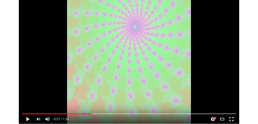](https://www.youtube.com/watch?v=X55JtZ7qRPM "geomandel demo video")
*Mandelbrot Fractal animated Zoom*
Besides the Mandelbrot Fractal geomandel supports the following other fractals:
* [Julia Set](https://en.wikipedia.org/wiki/Julia_set)
* [Tricorn](https://en.wikipedia.org/wiki/Tricorn_%28mathematics%29)
* [Burning Ship](https://en.wikipedia.org/wiki/Burning_Ship_fractal)
You may ask yourself how I came up with the name geomandel for this fractal
generator. Well my original plan was to play with fractals and GeoTIFFs to see
what kind of effects I could achieve with spatial geographic data. This is still
on my list of todos...
I also want to make you aware of the
[Mandelbrot project](https://github.com/willi-kappler/mandel-rust) a friend of
mine started. He uses Rust for his project and it motivated me to see how a C++11
solution would perform in comparison to his solution. I will provide some comparison
charts in the future.
## Features
* Generate Julia Sets, Tricorn, Burning Ship or Mandelbrot Fractals
* Set complex plane, bailout, and zoom coordinates / level
* Output calculated data as images (PNM / JPEG / PNG) or export as csv
* Different coloring algorithms
* Fast platform independent code written in C++11 using the cmake build system
## Setting up geomandel
In order to run the application on your system you either have to compile the
source code or use precompiled packages/installers.
### Source Code
To get the source code of the application
you may either download the [latest release](https://github.com/crapp/geomandel/releases/latest)
or you can check out the code from the [repository on github](https://github.com/crapp/geomandel).
Please use the master branch or one of the release branches.
In order to compile the source code on your machine the following requirements have to be met:
* cmake >= 3.2
* C++11 compliant compiler with proper ```std::regex``` support
* gcc >= 4.9
* clang >= 3.4
* MSVC >= 14 (Visual Studio 2015)
* MinGW >= 4.9
* [Simple and Fast Multimedia Library](http://www.sfml-dev.org/) for png/jpg support (optional)
The following external libraries are used by geomandel and are part of the
applications source code:
* [cxxopts](https://github.com/jarro2783/cxxopts) - Lightweight C++ command line option parser
* [CTPL](https://github.com/vit-vit/CTPL) - Modern and efficient C++ Thread Pool Library
* [Catch](https://github.com/philsquared/Catch) - A modern, C++-native, header-only, framework for unit-tests, TDD and BDD
#### Linux / OS X
Download and extract the source code. Enter the source code directory and use the
following commands to compile the application
```shell
# create a build directory and enter it
mkdir build
cd build
# run cmake to generate unix make files. Use -DUNIT_TEST=ON to build the
# unit tests application
cmake -DCMAKE_BUILD_TYPE=Release ../
# now compile the source code to create the geomandel executable. You can speed
# up compilation with the j option.
make
# optional run make install if you want to install the executable
make install
```
#### Windows
You can use the cmake Visual Studio Solution generator to compile the
application.
```shell
# create build directory and enter it
mkdir build
cd build
# assuming you are using Visual Studio 2015 on a 64bit Windows installation
# please change these options so they suit your build environment
cmake -G"Visual Studio 14 2015 Win64" ../
```
Open the solution file and compile the application.
Another possibility is to use the cmake NMake generator.
```shell
# create build directory and enter it
mkdir build
cd build
# check the prefix path so it matches your Qt installation
cmake -G"NMake Makefiles" ../
# build the application
nmake
```
### Precompiled packages, Installer
Precompiled Linux packages are available for
* Archlinux [](https://aur.archlinux.org/packages/geomandel)
## Usage
The command line application has sane default values for all options and you only
have to specify what kind of output you want to have. When the application is
started it will calculate the iteration count for all complex numbers in the complex
plane you defined. The iteration count can then be used to visualize the fractal
or the values can be exported to csv files. This is useful if you want to
test your own visualization algorithms.
### Command line options
geomandel uses the header only C++ command line parser [cxxopts](https://github.com/jarro2783)
The following command line options are available
```shell
Usage:
geomandel [OPTION...] - command line options
--help Show this help
-m, --multi [=arg(=2)] Use multiple cores
-q, --quiet Don't write to stdout (This does not influence
stderr)
Fractal options:
-f, --fractal arg Choose which kind of fractal you want to compute and
render (default:0)
-b, --bailout arg Bailout value for the fractal algorithm
(default:1000)
--creal-min arg Real part minimum (default:-2.0)
--creal-max arg Real part maximum (default:1.0)
--cima-min arg Imaginary part minimum (default:-1.5)
--cima-max arg Imaginary part maximum (default:1.5)
--julia-real arg Julia set constant real part (default:-0.8)
--julia-ima arg Julia set constant imaginary part (default:0.156)
Image options:
--image-file arg Image file name pattern. You can use different printf
like '%' items interspersed with normal text for the
output file name. Have a look in the README for more
instructions. (default:geomandel)
-w, --width arg Image width (default:1000)
-h, --height arg Image height (default:1000)
--image-pnm-bw Write Buffer to PBM Bitmap
--image-pnm-grey Write Buffer to grey scale PGM
--image-pnm-col Write Buffer to PPM Bitmap
--image-jpg Write Buffer to JPG image
--image-png Write Buffer to PNG image
--col-algo arg Coloring algorithm 0->Escape Time Linear,
1->Continuous Coloring Sine, 2->Continuous Coloring
Bernstein (default:1)
--grey-base arg Base grey color between 0 - 255 (default:55)
--grey-freq arg Frequency for grey shade computation (default:0.01)
--rgb-base arg Base RGB color as comma separated string
(default:128,128,128)
--rgb-freq arg Frequency for RGB computation as comma separated
string. You may use doubles but no negative values
(default:0.01,0.01,0.01)
--rgb-phase arg Phase for Sine Wave RGB computation as comma separated
string
(default:0,2,4)
--rgb-amp arg Amplitude for Bernstein RGB computation as comma
separated string (default:9,15,8.5)
--set-color arg Color for pixels inside the set (default:0,0,0)
--zoom arg Zoom level. Use together with xcoord, ycoord
--xcoord arg Image X coordinate where you want to zoom into the
fractal
--ycoord arg Image Y coordinate where you want to zoom into the
fractal
Export options:
-p, --print Print Buffer to terminal
--csv Export data to csv files
```
#### Fractal Options
In order to choose the fractal that will be computed the `--set` parameter exists.
The parameter has the following options:
```
--fractal=0 Mandelbrot Set (Default)
--fractal=1 Julia Set
--fractal=2 Tricorn
--fractal=3 Burning Ship
```
The complex plane is defined with these options:
```
--creal-min arg (-2.0)
--creal-max arg ( 1.0)
--cima-min arg (-1.5)
--cima-max arg ( 1.5)
```
You might need to adjust these values if you want to generate tricorn or julia
fractals.
In order to calculate the Julia Set a fixed constant is needed which you may provide
with `julia-real` and `julia-ima` (Default (-0.8+0.156i)).
The bailout value `bailout` defines the maximum amount of iterations used to
check whether a complex number is inside the Fractal. The higher you set
this value the more precise the predictions of the algorithm will be. But
computation time will also be significantly higher. The escape criterion, shown in
the pseudo code example below for the mandelbrot set, is not yet definable by a
command line parameter
(defaults to 2.0)
```c++
while ( x*x + y*y <= ESCAPE AND iteration < BAILOUT )
{
xtemp = x*x - y*y + x0
y = 2*x*y + y0
x = xtemp
iteration = iteration + 1
}
```
Computation speed can be reduced by using the ```multi``` option. This will
distribute the workload on different threads. See the *Performance* section for
more details.
One of the best features of Fractals is the possibility to zoom in indefinitely.
geomandel has specific convenient options to achieve this.
```
--zoom arg Zoom level. Use together with xcoord, ycoord
--xcoord arg Image X coordinate where you want to zoom into the fractal
--ycoord arg Image Y coordinate where you want to zoom into the fractal
```
The coordinates are image coordinates and describe the point where you want to zoom
into the fractal. Based on the coordinates and the zoom level a new complex plane
will be calculated. You can achieve the same effect if you use the complex plane
options directly but I think it is much easier to get the coordinates from an
image viewer and let geomandel do the math. All values can be decimals.
#### Image Options
geomandel is able to generate different image formats from the image algorithms.
How this images are generated can be influenced by command line parameters.
##### File name
The default output file name is geomandel + appropriate image format file extension.
You can use the `img-file` command line option which provides highly customizable
file names.
You can use different printf like '%' items interspersed with normal text for the
output file name. These items will be replaced by the application with the values
you chose.
```
%f Fractal name
%b Bailout value
%Zr Complex number real minimum
%ZR Complex number real maximum
%Zi Complex number imaginary minimum
%ZI Complex number imaginary maximum
%w Image width
%h Image height
%z Zoom level
%x Zoom x coordinate
%y Zoom y coordinate
```
If you have set a bailout value of 2048 and are using the default values for the
complex plane you could use a file name pattern like this
```
my_fractals_%bb_z(%Zr, %Zi)_z(%ZR, %ZI) -> my_fractals_2048b_z(-2.0, -1.5)_z(1.0, 1.5).[pgm|pbm|ppm|png|jpg]
```
Please note the naming scheme used for image files also applies for csv files
that will be generated when you use the ```csv``` command line option.
##### Image size
Use the following parameters to control the image size
```
-w, --width
-h, --height
```
These parameters have a large impact on memory footprint and computation time
##### Image formats
The application can generate images in the [portable anymap format (PNM)](https://en.wikipedia.org/wiki/Netpbm_format).
The big advantage of this format it is easy to implement and doesn't need any external
libraries. The downside is large files, as geomandel does not use a binary format, and
low writing speed.
You can choose between `img-pnm-bw` a simple black and white image, `img-pnm-grey`
using grey scale to render the fractal and `img-pnm-col` that generates
a RGB color image.
Additionally [SFML](http://www.sfml-dev.org/) can be used to generate jpg/png images.
These image formats use very little space on your disk and the library is quite fast.
You have to install the library and recompile geomandel if you want this kind of images.
##### Color Options
This is just a brief introduction into color command line options. See the **Color**
section for more information on this topic.
The `col-algo` parameter determines which coloring algorithm to use. Continuous
coloring can produce images without visible color bands. Computation time might
increase slightly though.
```
--col-algo arg Coloring algorithm 0->Escape Time Linear,
1->Continuous Coloring Sine, 2->Continuous Coloring Bernstein
```
Grey scale fractals are a nice alternative to colored ones. These parameters
control how the pgm images look like. The default value for grey scale frequency
is meant to be used with the linear escape time coloring algorithm.
```
--grey-base arg Base grey shade between 0 - 255
--grey-freq arg Frequency for grey shade computation
```
The RGB options apply to PPM as well as to PNG and JPG images. The base color
(background color) is set with `--rgb-base`. The distribution of the colors in
the color spectrum for the escape time or continuous index can be defined with
`--rgb-freq`, `--rgb-phase` and `--rgb-amp`. These options do different things
depending on the chosen coloring algorithm.
```
--rgb-base arg Base RGB color as comma separated string
--rgb-freq arg Frequency for RGB computation as comma separated
string. You may use decimals but no negative values
--rgb-phase arg Phase for Sine Wave RGB computation as comma separated string
--rgb-amp arg Amplitude for Bernstein RGB computation as comma separated string
```
The color of the pixels inside the fractal can be set with `set-color` command
line option.
### Examples
This section shows some examples of generated fractals and the command line
parameters necessary. Default values are used if not mentioned otherwise.
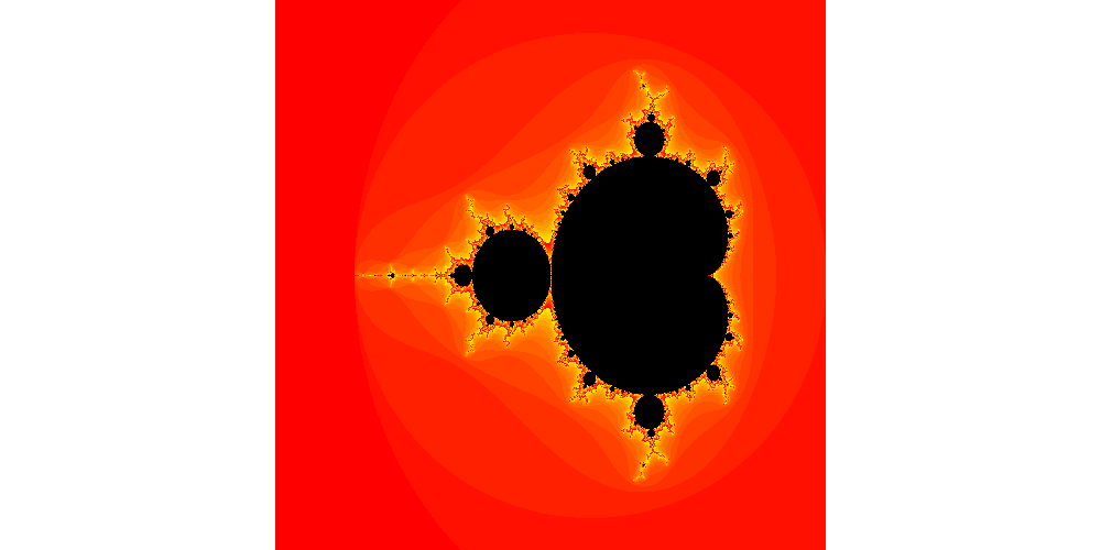
#### Mandelbrot fractal using linear escape time coloring
```shell
geomandel --col-algo=0 --rgb-freq=0,16,0 --rgb-base=255,0,0
```
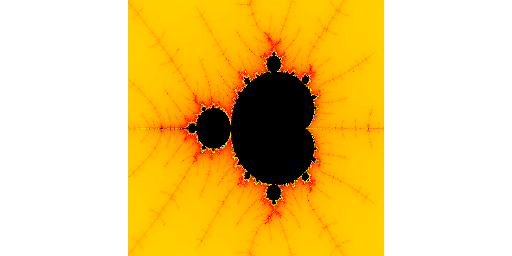
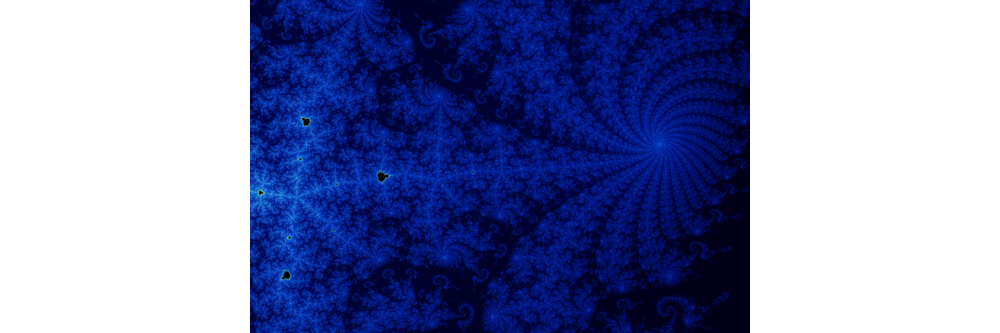
#### Mandelbrot fractal sine wave continuous coloring zoomed (200x)
```shell
geomandel --rgb-freq=0,0.01,0 --rgb-base=255,0,0 \
--xcoord=146 --ycoord=250 --zoom=200
```
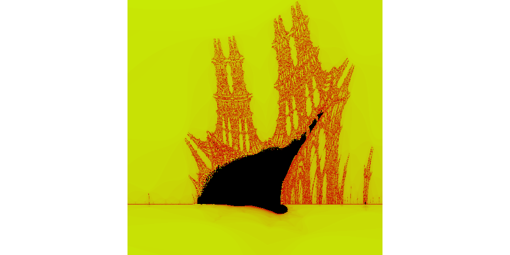
#### Burning Ship fractal sine wave
```shell
geomandel --fractal=3 --col-algo=1 \
--rgb-amp=0,7,0 --rgb-base=200,100,5 --rgb-freq=0,0.03,0 --rgb-phase=4,2,0 \
--xcoord=105.5 --ycoord=245 --zoom=30
```
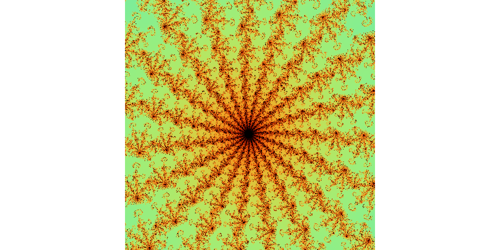
#### Zoomed Julia Fractal using continuous coloring based on Bernstein Polynomials
```shell
geomandel --fractal=2 --col-algo=2 --rgb-base=0,0,0 \
--creal-min=-1.5 --creal-max=1.8 \
--xcoord=253.5 --ycoord=289.7 --zoom=300
```
#### Full HD zoomed Mandelbrot Fractal, colored using Bernstein Polynomials
```shell
src/geomandel -w 1920 -h 1280 --image-png -m 4 -b 28000 \
--cima-min=-1.0 --cima-max=1.0 --creal-min=-2.0 \
--zoom=55250 --xcoord=471.42 --ycoord=615.681
```
[](https://crapp.github.io/geomandel/example_mandelbrot_zoomed_fullhd.png "Mandelbrot Full HD")
*Warning large image*
## Color
The fractal algorithms are well known and easy to implement. The more challenging
part is to draw beautiful fractals using different coloring algorithms. geomandel
offers different color strategies, escape time based linear and continuous coloring.
You can use the `col-algo` parameter too chose which one you want to apply.
### Escape Time Linear
The Escape Time linear algorithm is the most common method to color fractals. This is
because the method is fast, easy to understand and there are a lot of implementations
in the wild one can build on.
The pseudo code example in [command line options](#Mandelbrot-Options) section
shows how the escape time is calculated. geomandel takes this value and calculates
a RGB tuple or a grey scale value using the following formula

#### Grey Scale
Lets have a look at grey scale PGM images first. You can provide a base grey
shade with `grey-base` and a frequency value `grey-freq` which determines
how often sequences of grey shades repeat and their grading. This is best explained
with some images and plots.
The following Images and Plots were generated with `grey-base=55`
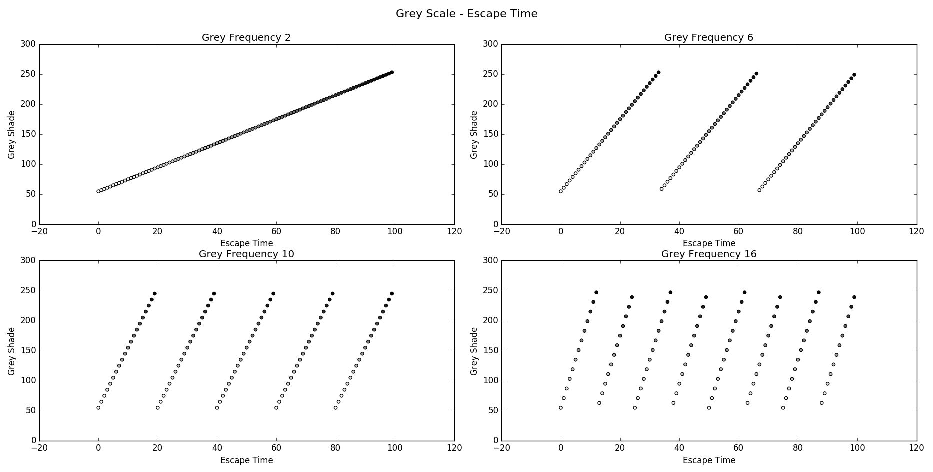
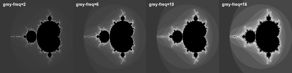
As you can see increasing the frequency will add better visual effects but also
worsens the problem of color banding.
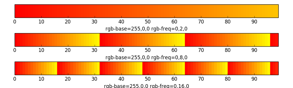
#### RGB Images
Generating RGB images with the Escape Time algorithm works similar to grey scale
images. You now have to use `rgb-base=R,G,B` to provide a base color and
`rgb-freq=FREQ_R,FREQ_G,FREQ_B` to determine the frequencies. Setting a
frequency to **0** will leave the respective color channel untouched.
The first three colorbars were created with a base color of `255,0,0` and a
RGB frequency of `0,2,0;0,8,0;0,16,0`. So only the green color component will
be changed.
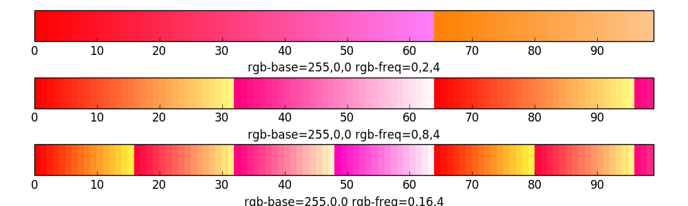
The next three colorbars were created with the same base color and the same frequency
values for the green channel. Additionally I have added a frequency of 4 for the
blue channel.
Here is what these values will look like as mandelbrot fractals.
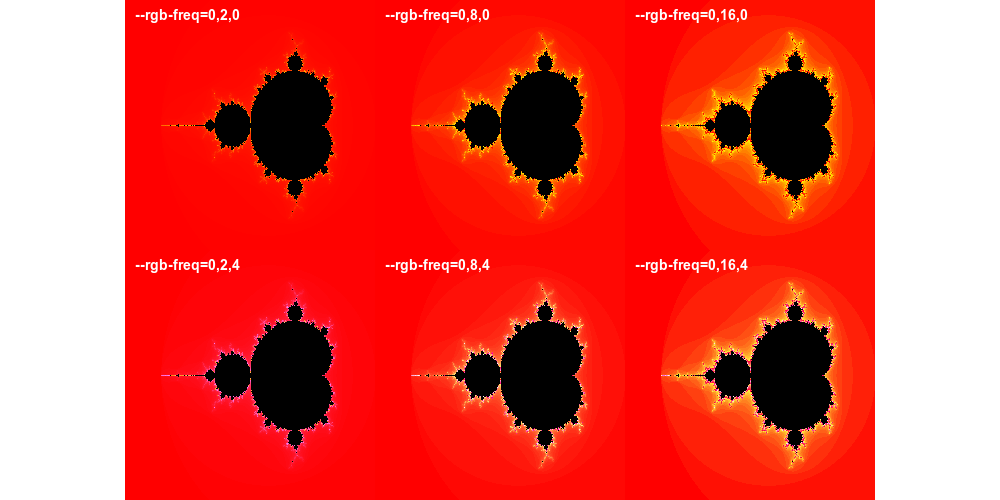
Feel free to experiment with these values to get the result you want. There is a
jupyter notebook `EscapeTimeRGB` in the resources folder that makes it easy to
visualize different values for RGB fractals generated with the escape time
algorithm.
### Continuous Coloring
Computing RGB values from the escape time in the fractal algorithms is easy but
has the disadvantage to produce visible color bands. This is because integer based
escape time consists of discrete values and this will result in a discrete color
scale. If the escape time is increased by 1 step we omit all values in between and
thus loosing the precision to color the fractal in a continuous way. Getting around
this is a bit more tricky and needs some additional computation steps.
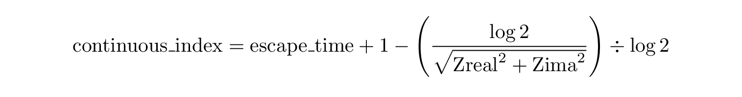
#### Mathematical Bases
A well known method is mapping the escape time on a logarithmic scale which will
give us a continuous gradient. Using a natural logarithm allows us to transform
the magnitude of every escaped pixel into a value between 0 and 1.
Here is the formula I use to calculate a continuous index for every complex number
of the complex plane.
Next step involves finding a good color map which colors blend smoothly and
of course endlessly as we can zoom a fractal indefinitely. Mathematical
functions used to model periodic and repeating phenomenas are the sine and
cosine functions. So a formula that uses out of phase sine functions to generate
real-time color blending could look like this:

Another method is to use a smooth polynomial that is defined on the unit interval
and has appropriate values. Slightly modified versions of the
[Bernstein polynomials](http://mathworld.wolfram.com/BernsteinPolynomial.html)
can be used as they are continuous, smooth and have values in the [0, 1] interval.
##### Sine wave based coloring
If you are interested in how this exactly works I highly recommend to read the article
about generating color sequences using sine and cosine by [Jim Bumgardner](http://krazydad.com/tutorials/makecolors.php). Reading this will help you understand how to use the options
`rgb-base`, `rgb-freq` and `rgb-phase` with the continuous sine coloring algorithm
to get the result you want.
As with escape time coloring using a frequency of 0 for a color component will
leave the appropriate base color channel untouched.
Here are some examples that show what you can achieve using this type of coloring.
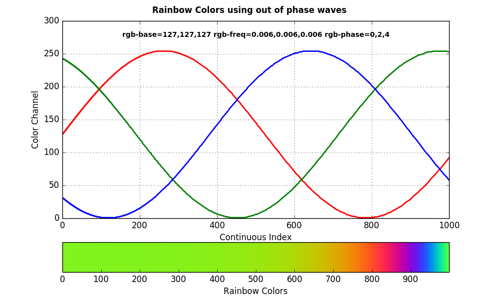
The first graph and colorbar show how you can get rainbow colors by using out of
phase color channel waves. If you would use the same phase and the same frequency
this would produce grey shades.
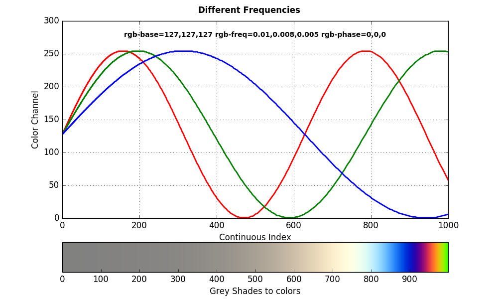
In the second example I used the same phase but different frequencies. If the base
color for all color channels is the same this will lead to a transition from
grey shades to colors.
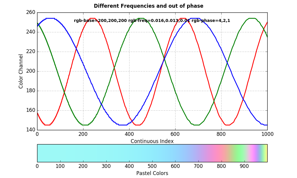
Interested in pastel colors? The last example shows exactly this using a higher
base color, different frequencies for the color channels and they are out of phase.
Choosing the right frequencies is highly dependent on the bailout value you used
for the fractal algorithm. If the frequencies are to high you will get color bands.
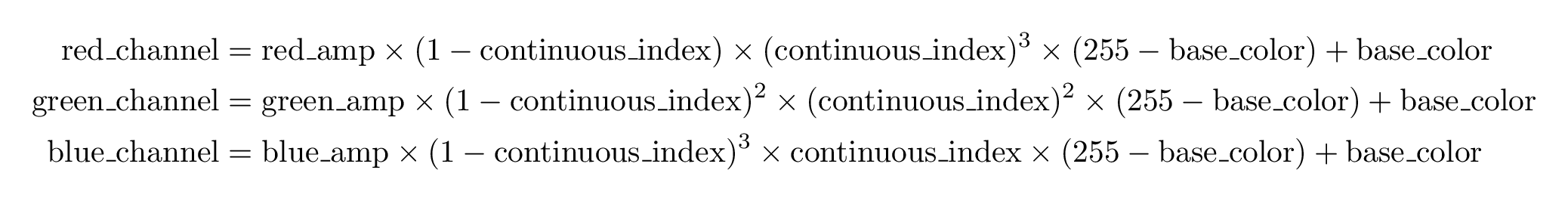
##### Bernstein polynomial based coloring
As I already mentioned Bernstein polynomials are continuous, smooth and have values
in the interval we need. Making them a good match to create RGB colors that blend
smoothly. You can use the parameters `rgb-base` and `rgb-amp`to influence this
coloring algorithm.
The base color is the background and starting color for this algorithm.
If you set the amplitude for a color channel to `0` the base color will not be
changed.
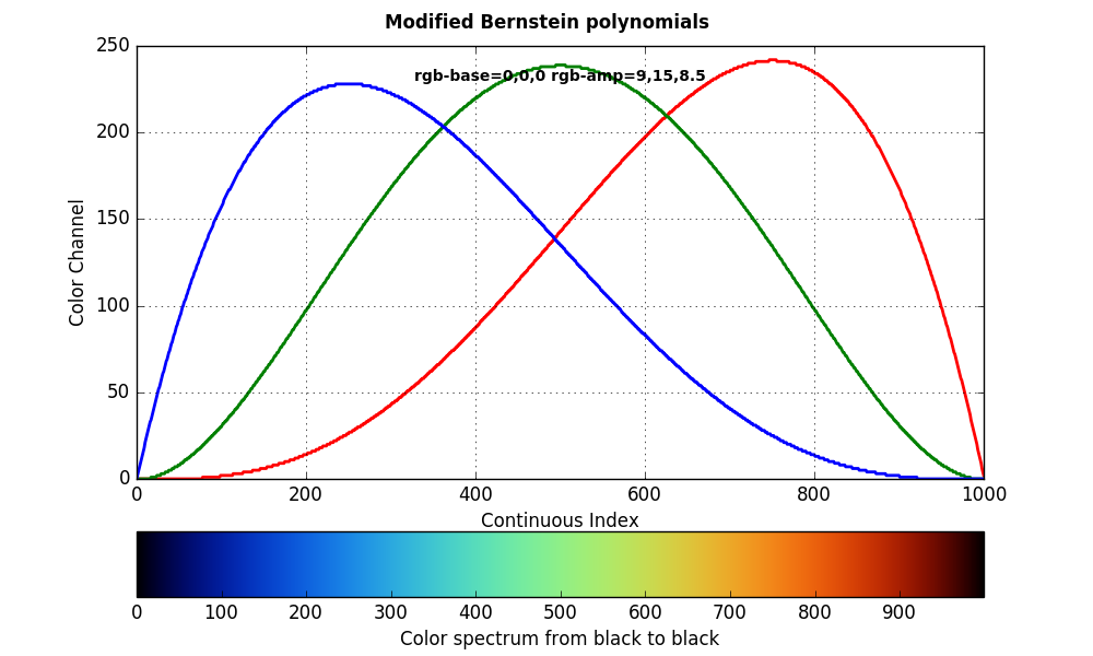
This graph shows you what colors you will get with a base color of `0, 0, 0`
and an amplitude of `9, 15, 8.5`
There is a jupyther notebook `BernsteinContinuousColoring` covering this coloring
algorithm in the resources folder.
## Performance and Memory usage
Calculating the escape time for a Mandelbrot Set is costly and may consume large
amounts of RAM. The computation benefits greatly from parallelism and it is easy
to distribute the workload accordingly. You can do this with the `--multi`
Parameter. geomandel will create the amount of threads specified by the multi
Parameter and uses the modern and efficient thread pool library
[CTPL](https://github.com/vit-vit/CTPL) to distribute the workload.
### Benchmarks

The chart shows how geomandel performs on different CPUs. The overhead seems to
be pretty small as doubling the number of threads nearly halves the time needed
for the computation.
While the Apple clang compiler generated binary performed as good as the gcc
binary on OS X (and even slightly better) the clang compiler on Linux is
outperformed by gcc by a factor of 2:1.
### Performance breakdown
Calculating the mathematical set of a fractal seems to be costly.
But how much time is really spend on computation? In order to answer this question
it is necessary to look at an application with a performance analyzing tool.
Luckily we have [perf](https://en.wikipedia.org/wiki/Perf_%28Linux%29) on Linux.

*Graph generated from perf data with gprof2dot*
As you can see ~97% of the applications CPU cycles were used to calculate a
mandelbrot set. Only one CPU core was used in this example.
So if you want to speed up this application this is the place to
start. I will try to maximize parallel computation with the use of GPUs in the
future for now you can use the `multi` option if your CPU offers multiple cores or
threads.
### Memory Footprint
The amount of memory used by geomandel is mostly dependant from image size and
image format. The internal buffer that stores the results of the fractal
number cruncher is preallocated at the beginning of the application. Therefor it
is simple to calculate the minimum amount of free memory you need to run geomandel.
The internal Buffer stores the modulus of the complex numbers (double) and the
escape time (int32).

As you can see in this equation you need around 12.6 MB for an image of the size
1024x1024. Of course this will be more in real life as I did not account for
[padding space](http://stackoverflow.com/a/937800/1127601) between data members
that is inserted by compilers to meet platform alignment requirements. In this
case 16 Bytes will be used meaning the application needs around 16 MB of free memory.
Lets see if valgrinds memory profiler [massif](http://valgrind.org/docs/manual/ms-manual.html)
is showing us the same values that I just calculated

*Memory profile derived from valgrinds massif tool*
Directly at the beginning the memory for the internal buffer is acquired and this
is close to my 16 MB assumption. At the end you can see another sharp rise in
memory usage. This is because I used SFML to generate a PNG image. SFML needs a
uint8_t data structure consisting of 4 bytes per pixel (RGBA). This leads to another
12 MB of memory acquired by geomandel. That comes to a total of ~28 MB of memory.
Please note this extra memory is only acquired when you use SFML (PNG/JPG).
## Development
Brief overview over the development process.
### Repositories
The [github repository](https://github.com/crapp/geomandel) of geomandel has
several different branches.
* master : Main development branch. Everything in here is guaranteed to
compile and is tested. This is the place for new features and bugfixes. Pull requests welcome.
* dev : Test branch and wild west area. May not compile.
* release-x.x : Branch for a release. Only bugfixes are allowed here. Pull requests welcome.
* gh-pages : Special branch for static HTML content hosted by github.io.
### Coding standards
The source code is formatted with clang-format using the following configuration
```
Language : Cpp,
BasedOnStyle : LLVM,
AccessModifierOffset : -4,
AllowShortIfStatementsOnASingleLine : false,
AlwaysBreakTemplateDeclarations : true,
ColumnLimit : 81,
IndentCaseLabels : false,
Standard : Cpp11,
IndentWidth : 4,
TabWidth : 4,
BreakBeforeBraces : Linux,
CommentPragmas : '(^ IWYU pragma:)|(^.*\[.*\]\(.*\).*$)|(^.*@brief|@param|@return|@throw.*$)|(/\*\*<.*\*/)'
```
### Versioning
I decided to use [semantic versioning](http://semver.org/)
### Unit Tests
I am using the great [Catch](https://github.com/philsquared/Catch) automated test framework.
Currently computation and command line parameters are covered by unit tests. This
will be expanded on coloring algorithms in the future.
To build the unit tests application use the cmake option ```-DUNIT_TEST=ON```
The unit tester can be run with `geomandel_test`. This will run all test cases and
output the result. See the Catch framework documentation for command line options
you can use to run only specific test cases, or change the application output.
### Continuous Integration
[](https://travis-ci.org/crapp/geomandel)
[Travis CI](https://travis-ci.org/) is used as continuous integration service.
The [geomandel github](https://github.com/crapp/geomandel) repository is linked
to Travis CI. You can see the build history for the master branch and all release
branches on the [travis project page](https://travis-ci.org/crapp/geomandel).
Besides testing compilation on different systems and compilers I also run the
unit tests after the application was compiled successfully.
## Bugs, feature requests, ideas
Please use the [github bugtracker](https://github.com/crapp/geomandel/issues)
to submit bugs or feature requests
## ToDo
Have a look in the todo folder. I am using the [todo.txt](http://todotxt.com/)
format for my todo lists.
## License
```
Copyright (C) 2015, 2016 Christian Rapp
This program is free software: you can redistribute it and/or modify
it under the terms of the GNU General Public License as published by
the Free Software Foundation, either version 3 of the License, or
(at your option) any later version.
This program is distributed in the hope that it will be useful,
but WITHOUT ANY WARRANTY; without even the implied warranty of
MERCHANTABILITY or FITNESS FOR A PARTICULAR PURPOSE. See the
GNU General Public License for more details.
You should have received a copy of the GNU General Public License
along with this program. If not, see <http://www.gnu.org/licenses/>.
```
Have a look into the license sub folder where license files of the used libraries
are located.