README.md

ggstream

The goal of ggstream is to create a simple but powerful implementation of streamplot/streamgraph in ggplot2. A streamplot is a stacked area plot mostly used for time series.

Installation

Install ggstream from CRAN:

install.packages("ggstream")

Or you can install the development version of ggstream from github with:

remotes::install_github("davidsjoberg/ggstream")

Examples

Type: Mirror

The characteristic streamplot which creates a symmetrical area chart around the x axis.

Type: Ridge

Which is equivalent to a stacked area chart.

Type: Proportional

The type proportional shows the share of each group in percent. Stacked like the ridge type.

Great community uses

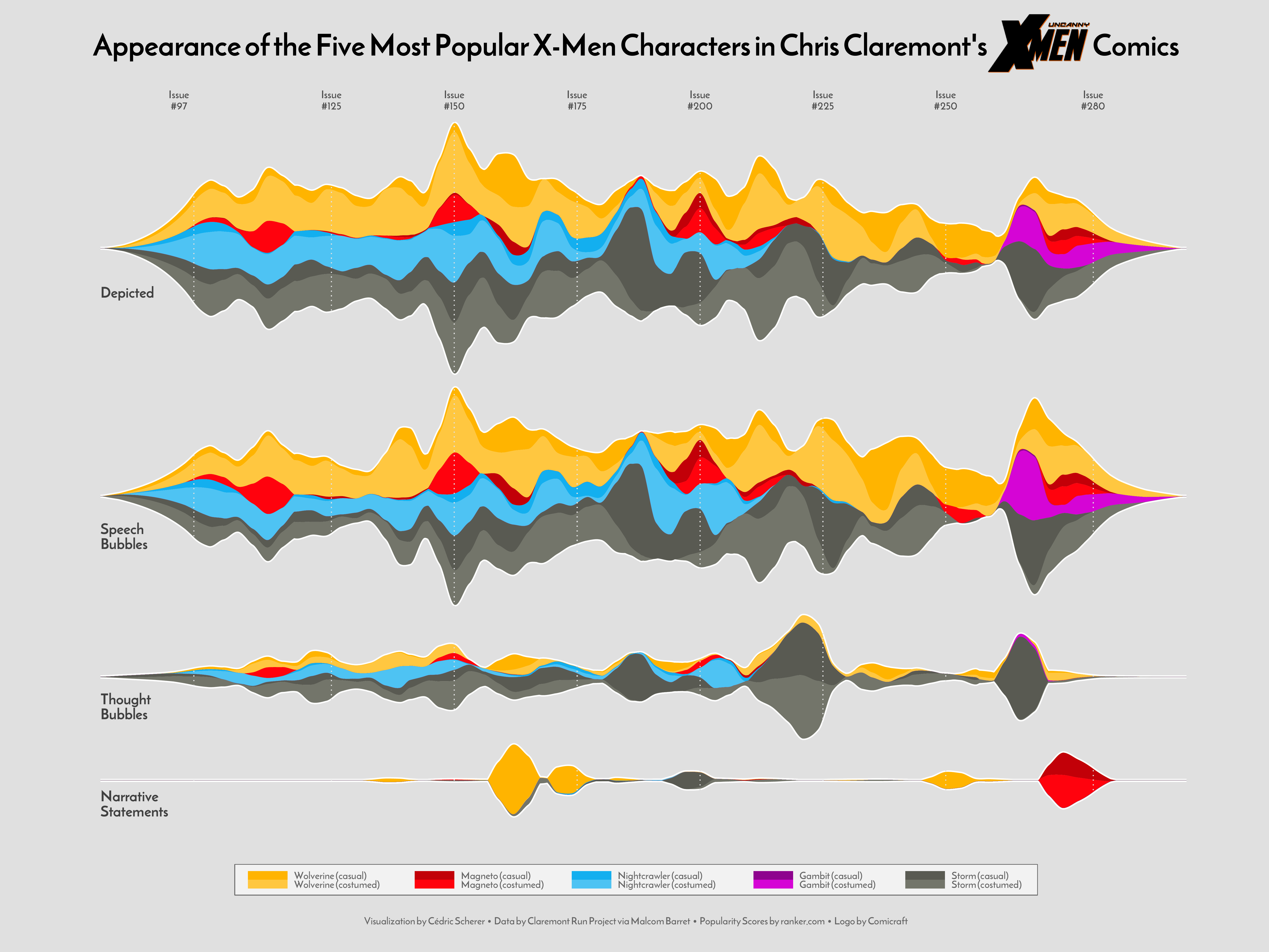By Cédric Scherer. Code here.

By Georgios Karamanis. Code here.

Basic usage

This is a basic example:

library(ggstream)

ggplot(blockbusters, aes(year, box_office, fill = genre)) +
  geom_stream()

ggstream also features a custom labeling geom that places decent default labels.

ggplot(blockbusters, aes(year, box_office, fill = genre)) +
  geom_stream() +
  geom_stream_label(aes(label = genre))

Add some pimp

library(cowplot)
library(paletteer)
library(dplyr)
library(colorspace)

blockbusters %>%
  ggplot(aes(year, box_office, fill = genre, label = genre, color = genre)) +
    geom_stream(extra_span = 0.013, type = "mirror", n_grid = 3000, bw = .78) +
    geom_stream_label(size = 4, type = "mirror", n_grid = 1000) +
  cowplot::theme_minimal_vgrid(font_size = 18) +
  theme(legend.position = "none") +
  scale_colour_manual(values = paletteer::paletteer_d("dutchmasters::milkmaid") %>% colorspace::darken(.8)) +
  scale_fill_manual(values = paletteer::paletteer_d("dutchmasters::milkmaid") %>% colorspace::lighten(.2)) +
  labs(title = "Box office per genre 1977-2019",
       x = NULL,
       y = "Current dollars, billions")

Advanced parameters

bw

The main parameter to adjust in geom_stream is probably the bandwidth, or bw. A lower bandwidth creates a more bumpy plot and a higher bandwidth smooth out some variation. Below is an illustration of how different bandwidths affect the stream plot.

library(patchwork)

base <- ggplot(blockbusters, aes(year, box_office, fill = genre)) + 
  theme(legend.position = "none")

(base +  geom_stream(bw = 0.5) + ggtitle("bw = 0.5")) /
(base +  geom_stream() + ggtitle("Default (bw = 0.75)")) /
(base +  geom_stream(bw = 1) + ggtitle("bw = 1"))

Extra Span

Another important parameter to adjust is extra_span. This parameter adjust if a larger range than the range of the data which can help if the edges of the stream plot grows too large due in the estimation function. The additional range is set to y = 0 which forces the area towards zero. The cut-off can include the extra range or fit the data. Too illustrate this rather unintuitive parameter some variations are shown below. The transparent areas show the full estimation, and the solid area is the final plot.

base <- ggplot(blockbusters, aes(year, box_office, fill = genre)) + 
  theme(legend.position = "none") +
  xlim(1970, 2028)

(base +  geom_stream() + ggtitle("Default")) /
(base +  geom_stream(extra_span = 0.001) + geom_stream(extra_span = 0.001, true_range = "none", alpha = .3) + ggtitle("extra_span = 0.001")) /
(base +  geom_stream(extra_span = .1) + geom_stream(extra_span = .1, true_range = "none", alpha = .3) + ggtitle("extra_span = .1")) /
(base +  geom_stream(extra_span = .2) + geom_stream(extra_span = .2, true_range = "none", alpha = .3) + ggtitle("extra_span = .2")) /
(base +  geom_stream(extra_span = .2, true_range = "none") + ggtitle("extra_span = .2 and true_range = \"none\""))

Sorting

Another feature of stream plots is the sorting of groups in the stacking. The default of ggstream is to stack as factor order of the fill aesthetics. However, ggstream supports two other stackning sorting options. The onset and inside_out.

library(patchwork)
set.seed(123)
df <- map_dfr(1:30, ~{
  x <- 1:sample(1:70, 1)
  tibble(x = x + sample(1:150, 1)) %>% 
    mutate(y = sample(1:10, length(x), replace = T),
           k = .x %>% as.character())
})

p <- df %>% 
  ggplot(aes(x, y, fill = k)) +
  theme_void() +
  theme(legend.position = "none")

p1 <- p + 
  geom_stream(color = "black") +
  ggtitle("None (Default)")

p2 <- p + geom_stream(color = "black", sorting = "inside_out") +
  ggtitle("Inside out")

p3 <- p +
  geom_stream(color = "black", sorting = "onset") +
  ggtitle("Onset")

p1 / p2 / p3

Final remarks

The ggstream package provides some flexible ways to make stream plots but with decent defaults. However, due to the complexity of the underlying smoothing/estimation it should be used carefully and mostly for fun too illustrate major trends.

If you find a bug or have ideas for additional feature you are more than welcome to open an issue.