50 Essential Autoencoders Interview Questions

You can also find all 50 answers here 👉 Devinterview.io - Autoencoders

1. What is an autoencoder?

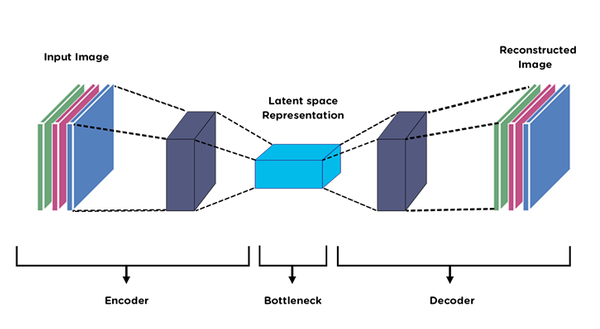
An autoencoder is a special type of neural network designed to learn efficient data representations, typically for unsupervised learning tasks. By compressing data into a lower-dimensional space and then reconstructing it, autoencoders can capture meaningful patterns within the data.

Core Components

• Encoder: Compresses input data into a lower-dimensional $z$ space. The encoder applies transformations, usually through a chain of layers, to map input data to a latent space.
• Decoder: Reconstructs the compressed data back to the original input space. This typically involves a layer architecture that mirrors the encoder but performs the reverse transformations.
• Latent Space Representation ($z$): Intermediate or bottleneck layer where data is compressed and from where the decoder generates the reconstruction.

Loss Function

The goal of training an autoencoder is to minimize the reconstruction error, which is often quantified using metrics like the mean squared error (MSE) between the input and the reconstructed output:

$$ \text{MSE} = \frac{1}{n} \sum_{i=1}^{n} (x_i - \text{Reconstructed}_i)^2 $$

Training Methodology

Autoencoders can be trained end-to-end using backpropagation in an unsupervised manner. By feeding the input data and its reconstruction to the network, you create a self-supervised learning setup. During training, the network aims to optimize the model by minimizing the reconstruction error.

Types of Autoencoders

1. Vanilla Autoencoder: It consists of a simple feedforward network and is trained to directly minimize reconstruction error.

2. Sparse Autoencoder: By enforcing sparsity in the latent space, these autoencoders encourage the model to learn more compact and meaningful representations.

3. Denoising Autoencoder: Trained to reconstruct clean data from noisy input, these models improve robustness and feature extraction.

4. Variational Autoencoder (VAE): Rather than producing a deterministic latent representation, VAEs model a probability distribution in the latent space and use generative sampling during training for better feature exploration. This method is particularly useful for generating new data points.

5. Convolutional Autoencoder: Ideal for handling image data, convolutional autoencoders use convolutional layers for both the encoder and decoder.

6. Recurrent Autoencoder: With the ability to handle sequential data, recurrent autoencoders leverage techniques such as Long Short-Term Memory (LSTM) layers for more effective data compression and reconstruction.

Use Cases

Since autoencoders are proficient in learning low-dimensional representations of complex data, they are valuable in various domains:

• Data Compression: By reducing the dimensionality of data, autoencoders efficiently compress information.

• Data Denoising: They can distinguish between noise and signal, useful in processing noisy datasets.

• Anomaly Detection: Autoencoders can identify deviations from normal or expected patterns, making them effective in fraud detection, medical diagnostics, and quality control.

• Data Visualization: By projecting high-dimensional data onto lower dimensions, such as 2D or 3D, autoencoders assist in data visualization tasks.

• Feature Engineering: Autoencoders are used to learn efficient feature representations, particularly when labeled data is scarce or unavailable.

• Data Generation: Certain autoencoder variants, such as VAEs, are capable of generating new data samples from the learned latent space, making them useful in generative tasks like image and text generation.

In summary, autoencoders are a versatile and powerful tool in the machine learning arsenal, especially for unsupervised learning and data preprocessing tasks.

2. Explain the architecture of a basic autoencoder.

An autoencoder is a type of artificial neural network used for unsupervised learning, where it learns to reconstruct input data. This is achieved via a bottleneck layer, a compressed representation of the input.

The basic architecture of an autoencoder comprises three key components:

1. Encoder: Responsible for reducing the input to a compressed representation.
2. Decoder: Reconstructs the input from the compressed representation.
3. Reconstruction Layer: Found at the output of the decoder, it aims to minimize the difference between the input and the reconstructed output.

Visual Representation

Key Components

1. Encoder: Combines a series of layers, typically feedforward neural network layers, to transform input data into a lower-dimensional representation. This transformation is the latent space and is often learned via techniques like backpropagation.

   • Input: The original data, most commonly flattened in vector form.
   • Layers: Multiple, can include dense, convolutional, or recurrent layers.
   • Output: Represents the latent space, usually a 1D or 2D vector.

2. Latent Space: It is a lower-dimensional space where the most salient features of the input data are represented. Its dimensionality can be controlled, but specific methods such as PCA or t-SNE are required for visualization.

3. Decoder: Reverse of the encoder, the decoder uses one or more feedback connections, sometimes referred to as "transposed" layers, to reconstruct the input. The number of neurons in the final layer matches the dimensionality of the input data.

   • Input: The compressed representation from the latent space.
   • Layers: Reversed structure of the encoder layers.
   • Output: Reconstructed input, usually homogeneous with the input data.

4. Reconstruction Loss Layer: Positioning of this layer is crucial; the optimization process aims to minimize the difference between the input data and the reconstructed output.

   • Loss: Often Mean Squared Error (MSE) or other appropriate metrics.
   • Output: Compares the reconstructed input with the original input to quantify the reconstruction error.

Usage in Feature Learning

Although initially designed for unsupervised learning and dimensionality reduction, autoencoders have demonstrated effectiveness in various tasks, including:

• Denoising: By training on noisy data, the autoencoder learns to remove noise.
• Anomaly Detection: It can identify outliers by detecting data points that are difficult to reconstruct.
• Feature Learning: It excels at learning salient representations or features in an unsupervised manner, which can then be used in supervised learning pipelines.

3. What is the difference between an encoder and a decoder?

In the context of autoencoders, both the encoder and the decoder play crucial roles, each accomplishing a specific task.

Their Distinct Functions

• Encoder: The encoder compresses input data into a more condensed form; in other words, it converts a high-dimensional input into a lower-dimensional one.

• Decoder: Its role is to reconstruct the original input data from the compressed representation produced by the encoder. It effectively "decodes" the reduced representation back into the original space.

Core Focus of Both Deigns

• Encoder: The encoder's emphasis is on distilling as much pertinent information as possible from the input.

• Decoder: The decoder focuses on generating output that matches the input as closely as feasible, remaining true to the input data's nuances.

4. How do autoencoders perform dimensionality reduction?

Autoencoders are neural networks that can perform unsupervised learning and nonlinear dimensionality reduction. By leveraging encoder and decoder components, they can learn effective, often nonlinear, data representations.

Many conventional dimensionality reduction methods, such as Principal Component Analysis (PCA), are linear. Autoencoders, by contrast, can learn more complex, nonlinear data structures.

The Mathematical Foundation

Autoencoders minimize a reconstruction loss that measures the difference between the input data and the output of the decoder. This process mathematically aligns with reducing reconstruction error in lower-dimensional subspaces.

More formally, the general idea is:

Given an input vector $x \in \mathbb{R}^n$, the autoencoder encodes it to $z \in \mathbb{R}^m$ such that $m < n$, then decodes it back to $x' \in \mathbb{R}^n$. The objective is to minimize the difference between $x$ and $x'$, usually defined by a metric like the Mean Squared Error (MSE).

Mathematically, the objective can be stated as:

$$ \min_{\text{Encoder},\text{Decoder}} | x - \text{Decoder}(\text{Encoder}(x)) |^2 $$

where $|\cdot|$ denotes a suitable norm.

Minimizing this objective results in a point-wise proximity between input and output data. Essentially, the autoencoder strives to reproduce its input as accurately as possible.

Visualizing Nonlinear Dimensionality Reduction

Conventional techniques, like PCA, identify a linear subspace that captures the most variance in the data. In contrast, autoencoders can uncover more intricate, nonlinear manifolds.

Consider the the 'Swiss roll' dataset, which is a 3-dimensional spiral unrolled into a 2-dimensional space.

Here is a plot that shows both traditional PCA and the autoencoder:

The PCA approach results in transitions that do not preserve the underlying structure, essentially causing the swiss roll to 'fold back' on itself in the flattened 2D space.

By contrast, the autoencoder, with its capacity to capture nonlinear relationships, faithfully reproduces the Swiss roll's structure in the reduced 2D space.

5. What are some key applications of autoencoders?

Autoencoders are a special type of neural network useful for non-linear dimensionality reduction and feature learning without supervision. Their unique architecture and training processes make them adaptable to a wide range of tasks.

Key Applications of Autoencoders

1. Data Denoising: Ideal for cleaning noisy input data. The network learns to eliminate random or systematic noise to reconstruct the original, clean input.

2. Anomaly Detection: By quantifying reconstruction error, autoencoders can identify input data that deviates significantly from normal, learned patterns. This technique is especially useful for fraud detection, network security, and industrial quality control.

3. Image Super-Resolution: Autoencoders can be trained to enhance image quality, a technique beneficial in medical imaging and photographic post-processing.

4. Domain Adaptation and Transfer Learning: They offer a robust approach to adapting a model trained over one domain of data to another, expedite training in some cases. For example, an autoencoder trained on synthetic data can help in training a classifier for real-world images.

5. Unsupervised Pre-training for Supervised Learning Tasks: Autoencoders can serve as a stepping stone for improving the performance of traditional classifiers by providing them with better, compressed, and more informative features.

6. Collaborative Filtering in Recommendation Systems: Autoencoders are instrumental in learning low-dimensional user and item representations from user-item interaction matrices in a recommendation system.

7. Feature Selector in Data Preprocessing: Employing the features learned by an autoencoder can be a suitable strategy for feature selection, helping reduce noise and redundancy in input data.

8. Generative Modeling: Autoencoders are instrumental in learning the underlying distribution of the input data and can be used to generate similar data samples. These reconstructed or synthetic samples can have various applications, such as text-to-image synthesis or video stabilization.

9. Embedding Visualization: They are useful for visualizing high-dimensional data in a lower-dimensional space; often, they are used for visualization and interpretability.

Code Example: Autoencoder for Data Denoising

Here is the Python code:

# Load Libraries
import numpy as np
import matplotlib.pyplot as plt
from keras.layers import Input, Dense
from keras.models import Model

# Generate Noisy Data
original_data = np.random.random((1000, 3))  # Example data
noise_factor = 0.5
noisy_data = original_data + noise_factor * np.random.normal(loc=0.0, scale=1.0, size=original_data.shape)

# Define Autoencoder
input_data = Input(shape=(3,))
encoded = Dense(2, activation='relu')(input_data)
decoded = Dense(3, activation='sigmoid')(encoded)
autoencoder = Model(input_data, decoded)
autoencoder.compile(optimizer='adam', loss='mean_squared_error')

# Train Autoencoder for Denoising
autoencoder.fit(noisy_data, original_data, epochs=50, batch_size=32, shuffle=True)

# Compare Original and Reconstructed Data
reconstructed_data = autoencoder.predict(noisy_data)

# Visualize Results
example_index = 0  # Choose any index
plt.scatter(original_data[example_index, 0], original_data[example_index, 1], c='b', label='Original')
plt.scatter(noisy_data[example_index, 0], noisy_data[example_index, 1], c='r', label='Noisy')
plt.scatter(reconstructed_data[example_index, 0], reconstructed_data[example_index, 1], c='g', label='Reconstructed')
plt.legend()
plt.show()

6. Describe the difference between a traditional autoencoder and a variational autoencoder (VAE).

Both autoencoders and variational autoencoders have distinct mechanisms for learning reduced or latent representations of input data.

Key Distinctions

• Nature of Encoded Inputs: The traditional autoencoder extracts a deterministic encoding. In contrast, the VAE learns a probabilistic distribution for each encoded input, typically Gaussian.

• Training Method: Autoencoders use deterministic mapping and straightforward backpropagation for training. VAEs, employing a probabilistic framework, employ variational methods.

• Latent Space Properties: Autoencoders generate a dense, continuous latent space. VAEs induce a latent space with specific statistical properties that enable sampling.

• Output Consistency: In most cases, autoencoders restore the input accurately. VAEs, due to their probabilistic nature, offer "approximate" and diverse reconstructions.

• Application in Data Generation: VAEs are generative models that can produce entirely new samples from the learned data distribution. Traditional autoencoders primarily reconstruct the input.

• Robustness to Noise: Autoencoders generally perform better (in terms of reconstruction) on noisy inputs.

• Limitations in Feature Generation: Although both architectures can be used to generate features, traditional autoencoders can suffer from their lack of structured, interpretable representations.

The VAE Sampling Process

To generate new data with a VAE, we sample from the learned latent space distribution for each feature of the input.

• Latent Space: Random samples are drawn from the learned multivariate Gaussian distribution.
• Decoder: These random samples are then passed through the decoder neural network to generate reconstructed outputs, which can be entirely novel images/text/other data types not seen during training.

This process leads to the generation of diverse outputs, a feature that's unique to VAEs and other generative models.

7. What is meant by the latent space in the context of autoencoders?

The latent space, also known as the coding space or bottleneck, is a core concept in autoencoder architectures. It describes the low-dimensional representation of input data, a compressed form that the encoder aims to optimize for and the decoder then aims to expand back to the input form.

In terms of the mathematical modeling, we can understand the latent space in the context of autoencoders as a mapping:

$$ \text{Encoder}: X \rightarrow Z $$

Where $X$ represents the input data and $Z$ represents the latent space, or the codings that represent the input data.

And the reverse can be said for the decoder:

$$ \text{Decoder}: Z \rightarrow \tilde{X} $$

Here, the mapping is from the latent space, $Z$, to a reconstructed form of the input data, $\tilde{X}$.

Key Concepts

1. Bottleneck Effect: Since autoencoders compress input data into a lower-dimensional space before reconstructing it, the structure maps to a bottleneck.

2. Latent Space Dimensionality: The number of dimensions in the latent space determines how much information the autoencoder can preserve.

3. Information Bottleneck Principle: This principle posits that the ideal latent space would strike a balance between retaining essential data and discarding noise.

4. Feature Learning: By leveraging unsupervised learning, autoencoders use the latent space to capture vital features from the data, like reconstructing numbers in a dataset like MNIST.

And in the decoder space, we're aiming to perform dimensionality expansion, meaning to create a reconstruction that's as close to the input as possible.

Once the encoder and decoder are trained, the autoencoder can make predictions in the latent space without relying on the decoder. Techniques like stochastic gradient descent and backpropagation are used during the training of an autoencoder to adjust the weights and biases in the network.

8. How can autoencoders be used for unsupervised learning?

Autoencoders are well-suited for unsupervised learning tasks as they can identify patterns and structures in unlabeled data. Let's learn about specific applications and techniques that leverage the capabilities of autoencoders.

Unsupervised Learning with Autoencoders

1. Data Compression: Autoencoders can distill the essential information from high-dimensional data, an essential step often preceding other machine learning tasks. For instance, compressed representations can be generated from raw imagery for tasks like object recognition.

2. Noise Removal: By obscuring portions of an image or text, autoencoders can learn to restore the original data, a process known as denoising. This technique is especially useful for tasks like image or audio reconstruction, where input data may be corrupted.

3. Anomaly Detection: Autoencoders can flag atypical data instances that don't conform to the majority of the training data. This method is particularly useful for spotting irregularities in datasets prone to having outliers.

4. Feature Learning: The hidden layers of an autoencoder can serve as rich feature extractors, making them invaluable in data representation tasks.

5. Recommendation Systems: Autoencoders can discern useful latent features from user-item interactions, effectively personalizing recommendations.

6. Dimensionality Reduction: By learning a reduced set of dimensions to describe the data, autoencoders excel in tasks where high-dimensionality is a challenge, such as for text data or spectrograms.

7. Inverse Problems: Meta-tasks like "restoring a corrupted image" or "filling in a missing piece of data" can be approached using autoencoders, thanks to their ability to generate data based on partial or problematic inputs.

9. Explain the concept of a sparse autoencoder.

A sparse autoencoder is an extension of the basic autoencoder, which introduces a regularization mechanism to promote sparsity in the learned latent representations. This is achieved through a sparsity constraint that makes the majority of the hidden units or neurons nearly inactive.

Mechanism Behind Sparsity Constraint

The aim is to have most hidden neurons close to 0, enforcing a \textbf{compression} of information.

Regularization Method

The autoencoder's cost function integrates an additional regularization term representing the KL divergence, a measure of the deviation of the hidden neurons' average activation from a target sparsity level.

The modified cost function:

$$ \mathcal{L}{\text{total}} = \mathcal{L}{\text{reconstruction}} + \lambda \sum_j \left( \rho \log\frac{\rho}{\hat{\rho}} + (1-\rho) \log\frac{1-\rho}{1-\hat{\rho}} \right) $$

Where:

• $\mathcal{L}_{\text{reconstruction}}$ is the reconstruction error
• $\lambda$ is the sparsity trade-off hyperparameter
• $\rho$ is the targeted sparsity level (e.g., 0.05 for 5%)
• $\hat{\rho}_j$ is the average activation of hidden unit $j$

Activation Functions

Choosing an appropriate activation function is crucial for ensuring the operation of the sparsity constraint. For example, specialized rectified linear units (ReLUs) such as the Kullback–Leibler (KL) divergence achieves sparsity control for encapsulating the activation function and the divergence term.

Training Strategies

Several methods exist for training sparse autoencoders, with the most common one being backpropagation. Throughout a backpropagation-based training process, AD controllers and simpler optimizers like SGD help adjust neuron activations and their average levels according to the sparsity constraint.

Practical Applications

Sparse autoencoders have seen success in various domains, such as anomaly detection, feature learning, and data visualization. Their ability to compress information through a reduced set of active neurons makes them an efficient choice for scenarios with limited data and computational resources.

10. What is a denoising autoencoder and how does it work?

A Denoising Autoencoder (DAE) is a type of autoencoder that's specifically trained to remove noise. This technique not only reconstructs clean data but also learns robust feature representations. This makes DAEs particularly useful in domains like computer vision and natural language processing, where input data is often noisy or incomplete.

Mechanism

A DAE consists of an encoder and a decoder, much like a standard autoencoder. However, during training, it's fed corrupted input (e.g., with added noise), and the objective is for the network to reconstruct the original, clean input. This introduces a form of regularization and encourages the model to learn representations that are less sensitive to noise.

Training Objective

The goal during training is to minimize the following reconstruction loss:

$$ L_{\text{reconstruct}} = \lVert X - D(E(X)) \rVert^{2} $$

Here, $X$ is the original input, $E(X)$ is the encoded (noisy) representation, and $D(E(X))$ is the decoded output, which ideally should be close to the original input.

DAE Advantages

• Noise Robustness: DAEs can effectively denoise and reconstruct noisy inputs, making them beneficial for real-world data.
• Unsupervised Learning: They learn representations without needing labeled data, making them versatile for various tasks.
• Regularization: The addition of noise during training acts as a form of regularization, reducing overfitting.

Practical Use-Cases

• Image Denoising: DAEs can clean up noisy images, enhancing their quality.
• Missing Data Handling: They are effective in scenarios where data might be missing or incomplete.
• Data Preprocessing: They can be integrated into pipelines for data preprocessing before feeding the data to more complex models.

Code Example: Denoising Autoencoder

Here is the Python code:

import numpy as np
import tensorflow as tf
from tensorflow.keras import layers, models

# Generate some noisy data for training
def generate_noisy_data(batch_size=64):
    clean_data = np.random.rand(batch_size, 100)
    noisy_data = clean_data + 0.1 * np.random.randn(batch_size, 100)  # Gaussian noise
    return noisy_data, clean_data

# Build denoising autoencoder
input_layer = layers.Input(shape=(100,))
encoded = layers.Dense(50, activation='relu')(input_layer)
decoded = layers.Dense(100, activation='sigmoid')(encoded)
dae = models.Model(input_layer, decoded)

# Compile and train the model
dae.compile(optimizer='adam', loss='mse')
noisy_data, clean_data = generate_noisy_data()
dae.fit(noisy_data, clean_data, epochs=10, batch_size=32)

11. Describe how a contractive autoencoder operates and its benefits.

A contractive autoencoder is a specialized type of autoencoder that augments the loss function with an additional penalty term. This results in a model that's trained to be robust to small input perturbations.

Contractive Autoencoder Mechanism

Core to a contractive autoencoder is its Jacobin matrix, which captures the impact of input perturbations on the hidden layer. This matrix is then squared element-wise and summed.

Mathematically, the core concept can be represented as:

$$ \text{J}(\mathbf{x}) = \frac{\partial \mathbf{h}(\mathbf{x})}{\partial \mathbf{x}} = \left( \frac{\partial h_i(\mathbf{x})}{\partial x_j} \right)_{i, j} $$

The contractive term, added to the loss function, is defined as the Frobenius norm of the Jacobian matrix (L2 norm of the matrix, treated as a vector). The higher its value, the more the model is penalized for its sensitivity to input perturbations.

$$ L_{contractive} = \sum_{ij} \left( \frac{\partial h_i(\mathbf{x})}{\partial x_j} \right)^2 $$ $$ L_{total} = L_{reconstruction} + \alpha L_{contractive} $$

Key Benefits

1. Regularization: The added contractive loss term serves as a form of regularization. This technique can benefit data-limited scenarios or when the data is inherently noisy.

2. Improved Robustness: The loss function encourages the autoencoder to produce hidden-layer representations that are stable, even with slight variations in input. This stability often leads to better generalization and robustness of the model.

3. Unsupervised Feature Learning: As with standard autoencoders, the hidden layer of a contractive autoencoder can capture intrinsic features of the input data. The contractive term, while adding regularization, does not mandate explicit supervision.

4. Data Compression and De-Noising: Autoencoders, including their contractive variation, maintain their fundamental utility as tools for both dimensionality reduction and de-noising tasks.

Code Example: Contractive Autoencoder

Here is the Python Keras code:

from keras import layers, models, regularizers

# Build the contractive autoencoder
input_data = layers.Input(shape=(input_dim,))
encoded = layers.Dense(encoding_dim, activation='relu', activity_regularizer=regularizers.l2(10e-5))(input_data)
decoded = layers.Dense(input_dim, activation='sigmoid')(encoded)

# Compile the model, specifying the loss function and optimizer
contractive_ae = models.Model(input_data, decoded)
contractive_ae.compile(optimizer='adam', loss='binary_crossentropy')

# Train the model
contractive_ae.fit(train_data, train_data, epochs=100, batch_size=256, shuffle=True, validation_data=(test_data, test_data))

12. What are convolutional autoencoders and in what cases are they preferred?

A Convolutional Neural Network (CNN) is designed to handle visual data by implementing convolutional layers which 'scan' input images to learn local features. Conversely, an autoencoder is a neural network that employs an encoder to reduce data dimensions and a decoder to reconstruct the original data.

A Convolutional Autoencoder combines both these concepts to facilitate dimensionality reduction and image reconstruction using convolutional layers.

Key Components of a Convolutional Autoencoder

• Encoder Utilizes convolutional layers, pooling, and possibly other techniques such as batch normalization and activation layers to reduce the input's dimensionality. Convolutional layers scan the input, identifying key features that are then downsampled through pooling layers.

• Decoder This section includes transposed convolutions (deconvolutions), which expand the feature maps back to their original size. As a result, a reconstructed image that is visually close to the input. These layers act as upscaling mechanisms that restore finer details. The final layer typically uses a sigmoid or hyperbolic tangent function to ensure pixel values fall within the range of 0 to 1.

• Loss Function Commonly, mean squared error (MSE) or binary cross-entropy is employed to gauge the difference between the original input and the generated output. The objective is to minimize this difference during training.

This architecture allows for learning useful image representations and, with the added benefit of being able to handle variable-sized images.

13. How do recurrent autoencoders differ from feedforward autoencoders, and when might they be useful?

Recurrent Autoencoders (RAEs) combine the benefits of both Recurrent Neural Networks (RNNs) and Autoencoders, making them particularly suitable for sequential data.

Key Distinction

• Feedback Mechanism: Unlike Feedforward Autoencoders (FAEs) that are designed for static data, RAEs handle evolving sequences by leveraging the feedback loops in RNNs.

This dynamic capability allows them to serve well in tasks reliant on chronological order.

Unique Features of Recurrent Autoencoders

1. Context Preservation: Ideal for applications where sequence context is crucial, such as in natural language processing for tasks like text completion or translation.

2. Capacity for Variable-Length Input/Output: Adaptable to data with changing sizes or sequences, obviating the need for fixed-size inputs or outputs.

3. GED Limitations Mitigation: Overcome the limitations related to the General Edit Distance (GED), like those frequently encountered in speech recognition, by offering more precise and context-aware embeddings for sequences.

4. Stateful Embeddings: Create embeddings designed to preserve contextual memory.

Practical Applications

1. Speech Recognition: Supporting tasks such as automatic speech recognition (ASR) in which the temporal nature of speech data is fundamental.

2. Feature Learning: Proficient in capturing crucial temporal features in applications like ECG signal analysis or stock market predictions.

3. Information Retrieval on Time-Evolving Data: Suitable for indexing and querying real-time sequential data, such as for streaming text or news articles.

4. Video Data Processing: Handling of varied video content, from action recognition to generating descriptions.

5. Text Data Analysis and Generation: Effective in sequential text-based tasks like text summarization or generating structured responses.

14. Explain the idea behind stacked autoencoders.

Stacked Autoencoders (SAEs) are an advanced variation of autoencoders that use a series of multiple connected autoencoders for progressive feature extraction and non-linear dimensionality reduction. SAEs have several applications, including unsupervised pre-training for deep neural networks, and are often used as building blocks for more complex systems such as Restricted Boltzmann Machines.

Progressive Feature Extraction

The primary goal of an SAE is to learn a hierarchy of increasingly abstract representations of the input data, much like a deep neural network. Each autoencoder layer functions as a feature extractor, refining the input at each step.

The key to the success of this approach is in training the stacked autoencoders in stages, which helps overcome the limitations of using a single, large autoencoder.

Training Mechanism

The input data is preprocessed by the first autoencoder, and the resulting encoded representation becomes the input to the next autoencoder in the stack. This process is carried out through all the layers of the stacked autoencoders.

The network is trained one layer at a time to simplify the learning process, typically using unsupervised learning techniques like the backpropagation algorithm.

After training each layer, the network is combined, essentially treating all the layers after the first as a single, deep autoencoder. This combined network is further fine-tuned through backpropagation using the original, unprocessed input data.

Challenges and Advantages

Challenges

• Vanishing Gradient: As training progresses from the first layer to the last, gradients can diminish, making the earlier layers hard to train. Techniques like layer-wise pre-training can alleviate this.

• Overfitting: Deeper networks are prone to overfitting. It's crucial to employ techniques like regularization.

• Hyperparameter Sensitivity: SAEs require delicate balance among several hyperparameters, making their optimization challenging.

Advantages

• Improved Generalization: By learning manifold structures and avoiding local minima, SAEs often lead to better representations.

• Deeper Layers Benefit: Unlike shallow autoencoders, SAEs can harness learning from multiple layers, leading to superior categorical and invariant features.

• Useful for Various Tasks: SAEs can be employed for both unsupervised and semi-supervised learning tasks.

Code Example: Unsupervised Pre-Training for z-Dimension Selection

Here is the Python code:

from keras.layers import Input, Dense
from keras.models import Model

# Create the stacked autoencoder
input_data = Input(shape=(784,))
encoder1 = Dense(256, activation='relu')(input_data)
encoder2 = Dense(128, activation='relu')(encoder1)
decoder1 = Dense(256, activation='relu')(encoder2)
decoded = Dense(784, activation='sigmoid')(decoder1)

# Train the first autoencoder
autoencoder1 = Model(input_data, decoder1)
# ... Compile with optimizer and loss function, then fit on input_data

# Train the overall autoencoder network with fine-tuning
autoencoder2 = Model(input_data, decoded)
# ... Compile with optimizer and loss function, then fit on input_data

15. Discuss the role of regularization in training autoencoders.

Autoencoders usually undergo unsupervised learning and can also benefit from regularization techniques to enhance generalization. Regularization helps to address overfitting, especially in scenarios with limited training data.

Common Regularization Methods in Autoencoders

1. L1 and L2 Regularization: These methods add a penalty term to loss functions, making models less sensitive to noise in input data. L1 regularization encourages sparsity—eliminating some inputs entirely from the network—while L2 promotes small weight coefficients.

2. Dropout: Often employed in deep neural networks, dropout randomly sets a fraction of the neuron activations to zero during training, minimizing the reliance on specific features.

3. Noise Injection: Introducing random noise during training can also improve network generalization. Common techniques include data perturbation (e.g., adding noise to input samples) and injecting noise directly into the hidden layers.

4. Data Augmentation: Widely used in supervised learning, data augmentation techniques could also benefit unsupervised setups such as autoencoders. By increasing the diversity of training samples—be it through rotations, translations, or other transformations—these methods can help the network extract more robust features.

Code Example: L2 Regularization in Keras

Here is the Python code:

import numpy as np
import tensorflow as tf
from tensorflow.keras import layers, models, regularizers

# Sample dataset (2D data)
X = np.random.rand(100, 2)

# Define the autoencoder
input_dim = X.shape[1]
encoding_dim = 1

input_layer = layers.Input(shape=(input_dim,))
encoded = layers.Dense(encoding_dim, activation='linear', activity_regularizer=regularizers.l2(0.01))(input_layer)
decoded = layers.Dense(input_dim, activation='linear')(encoded)

autoencoder = models.Model(input_layer, decoded)

# Compile the autoencoder
autoencoder.compile(optimizer='adam', loss='mean_squared_error')

# Train the autoencoder
autoencoder.fit(X, X, epochs=100, batch_size=16)

Explore all 50 answers here 👉 Devinterview.io - Autoencoders