Dynamic Time Warping based Hierarchical Agglomerative Clustering

• For details, see the research paper: On analyzing GNSS displacement field variability of Taiwan: Hierarchical Agglomerative Clustering based on Dynamic Time Warping technique
• Codes to perform Dynamic Time Warping Based Hierarchical Agglomerative Clustering of GPS data

Documentation

Installation and usage information can be obtained from the documentation: dtwhaclustering.pdf

Complete documentation at: dtwhaclustering-docs

Details

This package include codes for processing the GPS displacement data including least-square modelling for trend, co-seismic jumps, seasonal and tidal signals. Finally, it can be used to cluster the GPS displacements based on the similarity of the waveforms. The similarity among the waveforms will be obtained using the DTW distance.

Usage

Least-squares modeling

from dtwhaclustering.leastSquareModeling import lsqmodeling
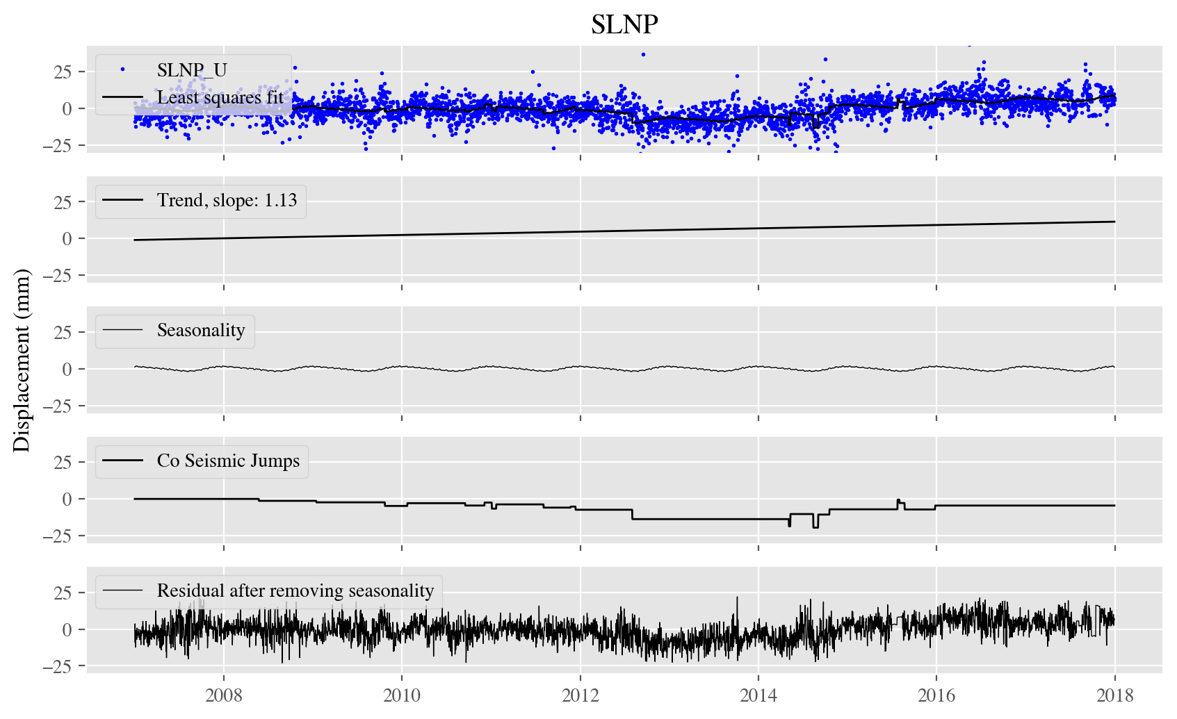
final_dU, final_dN, final_dE = lsqmodeling(dUU, dNN, dEE,stnlocfile="helper_files/stn_loc.txt",  plot_results=True, remove_trend=False, remove_seasonality=True, remove_jumps=False)

Plot station map

from dtwhaclustering import plot_stations
plot_stations.plot_station_map(station_data = 'helper_files/selected_stations_info.txt', outfig=f'{outloc}/station_map.pdf')

Plot linear trend

slopeFile=f'stn_slope_res_U.txt'
df = pd.read_csv(slopeFile, names=['stn','lon','lat','slope'], delimiter='\s+')
plot_linear_trend_on_map(df, outfig=f"Maps/slope-plot_U.pdf")

Note: slopeFile is obtained from lsqmodeling.

Dynamic Time Warping Analysis

from dtwhaclustering.dtw_analysis import dtw_signal_pairs, dtw_clustering
import numpy as np
from scipy import signal
import matplotlib.pyplot as plt

np.random.seed(0)
# sampling parameters
fs = 100   # sampling rate, in Hz
T = 1      # duration, in seconds
N = T * fs  # duration, in samples

# time variable
t = np.linspace(0, T, N)

SNR = 0.2 #noise

XX0 = np.sin(2 * np.pi * t * 7+np.pi/2) #+ np.random.randn(1, N) * SNR
XX1 = signal.sawtooth(2 * np.pi * t * 5+np.pi/2) #+ np.random.randn(1, N) * SNR
# XX1 = np.abs(np.cos(2 * np.pi * t * 3)) - 0.5
s1, s2 = XX0, XX1

dtwsig = dtw_signal_pairs(s1, s2, labels=['S1', 'S2'])

dtwsig.plot_signals()
plt.show()

dtwsig.plot_matrix(windowfrac=0.6, psi=None) #Only allow for shifts up to 60% of the minimum signal length away from the two diagonals.
plt.show()

References

1. Kumar, U., Chao, B.F., Chang, E.T.-Y.Y., 2020. What Causes the Common‐Mode Error in Array GPS Displacement Fields: Case Study for Taiwan in Relation to Atmospheric Mass Loading. Earth Sp. Sci. 0–2. https://doi.org/10.1029/2020ea001159

Please cite this work as

1. Kumar, U., Cédric. P. Legendre, Jian-Cheng Lee, Li Zhao, Benjamin Fong Chao (2022) On analyzing GNSS displacement field variability of Taiwan: Hierarchical Agglomerative Clustering based on Dynamic Time Warping technique Computers & Geosciences, 105243. https://doi.org/10.1016/j.cageo.2022.105243
2. Kumar, U., Legendre, C.P. (2022) Crust-mantle decoupling beneath Afar revealed by Rayleigh-wave tomography Sci Rep 12, 17036 https://doi.org/10.1038/s41598-022-20890-5

License

© 2021 Utpal Kumar

Licensed under the Apache License, Version 2.0