/
nlp_estimators.py
448 lines (322 loc) · 27.3 KB
/
nlp_estimators.py
1
2
3
4
5
6
7
8
9
10
11
12
13
14
15
16
17
18
19
20
21
22
23
24
25
26
27
28
29
30
31
32
33
34
35
36
37
38
39
40
41
42
43
44
45
46
47
48
49
50
51
52
53
54
55
56
57
58
59
60
61
62
63
64
65
66
67
68
69
70
71
72
73
74
75
76
77
78
79
80
81
82
83
84
85
86
87
88
89
90
91
92
93
94
95
96
97
98
99
100
101
102
103
104
105
106
107
108
109
110
111
112
113
114
115
116
117
118
119
120
121
122
123
124
125
126
127
128
129
130
131
132
133
134
135
136
137
138
139
140
141
142
143
144
145
146
147
148
149
150
151
152
153
154
155
156
157
158
159
160
161
162
163
164
165
166
167
168
169
170
171
172
173
174
175
176
177
178
179
180
181
182
183
184
185
186
187
188
189
190
191
192
193
194
195
196
197
198
199
200
201
202
203
204
205
206
207
208
209
210
211
212
213
214
215
216
217
218
219
220
221
222
223
224
225
226
227
228
229
230
231
232
233
234
235
236
237
238
239
240
241
242
243
244
245
246
247
248
249
250
251
252
253
254
255
256
257
258
259
260
261
262
263
264
265
266
267
268
269
270
271
272
273
274
275
276
277
278
279
280
281
282
283
284
285
286
287
288
289
290
291
292
293
294
295
296
297
298
299
300
301
302
303
304
305
306
307
308
309
310
311
312
313
314
315
316
317
318
319
320
321
322
323
324
325
326
327
328
329
330
331
332
333
334
335
336
337
338
339
340
341
342
343
344
345
346
347
348
349
350
351
352
353
354
355
356
357
358
359
360
361
362
363
364
365
366
367
368
369
370
371
372
373
374
375
376
377
378
379
380
381
382
383
384
385
386
387
388
389
390
391
392
393
394
395
396
397
398
399
400
401
402
403
404
405
406
407
408
409
410
411
412
413
414
415
416
417
418
419
420
421
422
423
424
425
426
427
428
429
430
431
432
433
434
435
436
437
438
439
440
441
442
443
444
445
446
447
448
# -*- coding: utf-8 -*-
"""nlp_estimators.ipynb
Automatically generated by Colaboratory.
Original file is located at
https://colab.research.google.com/drive/1oXjNYSJ3VsRvAsXN4ClmtsVEgPW_CX_c
Classifying text with TensorFlow Estimators
===
This notebook demonstrates how to tackle a text classification problem using custom TensorFlow estimators, embeddings and the [tf.layers](https://www.tensorflow.org/api_docs/python/tf/layers) module. Along the way we'll learn about word2vec and transfer learning as a technique to bootstrap model performance when labeled data is a scarce resource.
## Setup
Let's begin importing the libraries we'll need. This notebook runs in Python 3 and TensorFlow v1.4 or more, but it can run in earlier versions of TensorFlow by replacing some of the import statements to the corresponding paths inside the `contrib` module.
### The IMDB Dataset
The dataset we wil be using is the IMDB [Large Movie Review Dataset](http://ai.stanford.edu/~amaas/data/sentiment/), which consists of $25,000$ highly polar movie reviews for training, and $25,000$ for testing. We will use this dataset to train a binary classifiation model, able to predict whether a review is positive or negative.
"""
import os
import string
import tempfile
import tensorflow as tf
import numpy as np
import matplotlib.pyplot as plt
from tensorflow.python.keras.datasets import imdb
from tensorflow.python.keras.preprocessing import sequence
from tensorboard import summary as summary_lib
tf.logging.set_verbosity(tf.logging.INFO)
print(tf.__version__)
"""### Loading the data
Keras provides a convenient handler for importing the dataset which is also available as a serialized numpy array `.npz` file to download [here]( https://s3.amazonaws.com/text-datasets/imdb.npz). Each review consists of a series of word indexes that go from $4$ (the most frequent word in the dataset, **the**) to $4999$, which corresponds to **orange**. Index $1$ represents the beginning of the sentence and the index $2$ is assigned to all unknown (also known as *out-of-vocabulary* or *OOV*) tokens. These indexes have been obtained by pre-processing the text data in a pipeline that cleans, normalizes and tokenizes each sentence first and then builds a dictionary indexing each of the tokens by frequency. We are not convering these techniques in this post, but you can take a look at [this chapter](http://www.nltk.org/book/ch03.html) of the NLTK book to learn more.
"""
vocab_size = 5000
sentence_size = 200
embedding_size = 50
model_dir = tempfile.mkdtemp()
# Should we not use keras and rewrite this logic?
print("Loading data...")
(x_train_variable, y_train), (x_test_variable, y_test) = imdb.load_data(
num_words=vocab_size)
print(len(y_train), "train sequences")
print(len(y_test), "test sequences")
print("Pad sequences (samples x time)")
x_train = sequence.pad_sequences(x_train_variable,
maxlen=sentence_size,
padding='post',
value=0)
x_test = sequence.pad_sequences(x_test_variable,
maxlen=sentence_size,
padding='post',
value=0)
print("x_train shape:", x_train.shape)
print("x_test shape:", x_test.shape)
"""We can use the word index map to inspect how the first review looks like."""
word_index = imdb.get_word_index()
word_inverted_index = {v: k for k, v in word_index.items()}
# The first indexes in the map are reserved to represet things other than tokens
index_offset = 3
word_inverted_index[-1 - index_offset] = '_' # Padding at the end
word_inverted_index[ 1 - index_offset] = '>' # Start of the sentence
word_inverted_index[ 2 - index_offset] = '?' # OOV
word_inverted_index[ 3 - index_offset] = '' # Un-used
def index_to_text(indexes):
return ' '.join([word_inverted_index[i - index_offset] for i in indexes])
print(index_to_text(x_train_variable[0]))
"""## Building Estimators
In the next section we will build several models to make predictions for the labels in the dataset. We will first use canned estimators and then create custom ones for the task. We recommend that you check out [this blog post](https://developers.googleblog.com/2017/11/introducing-tensorflow-feature-columns.html) that explains how to use the `tf.feature_column` module to standardize and abstract how raw input data is processed and [the following one](https://developers.googleblog.com/2017/12/creating-custom-estimators-in-tensorflow.html) that covers in depth how to work with Estimators.
### From arrays to tensors
There's one more thing we need to do get our data ready for TensorFlow. We need to convert the data from numpy arrays into Tensors. Fortunately for us the `Dataset` module has us covered.
It provides a handy function, `from_tensor_slices` that creates the dataset to which we can then apply multiple transformations to shuffle, batch and repeat samples and plug into our training pipeline. Moreover, with just a few changes we could be loading the data from files on disk and the framework does all the memory management.
We define two input functions: one for processing the training data and one for processing the test data. We shuffle the training data and do not predefine the number of epochs we want to train, while we only need one epoch of the test data for evaluation. We also add an additional `"len"` key to both that captures the length of the original, unpadded sequence, which we will use later.
"""
x_len_train = np.array([min(len(x), sentence_size) for x in x_train_variable])
x_len_test = np.array([min(len(x), sentence_size) for x in x_test_variable])
def parser(x, length, y):
features = {"x": x, "len": length}
return features, y
def train_input_fn():
dataset = tf.data.Dataset.from_tensor_slices((x_train, x_len_train, y_train))
dataset = dataset.shuffle(buffer_size=len(x_train_variable))
dataset = dataset.batch(100)
dataset = dataset.map(parser)
dataset = dataset.repeat()
iterator = dataset.make_one_shot_iterator()
return iterator.get_next()
def eval_input_fn():
dataset = tf.data.Dataset.from_tensor_slices((x_test, x_len_test, y_test))
dataset = dataset.batch(100)
dataset = dataset.map(parser)
iterator = dataset.make_one_shot_iterator()
return iterator.get_next()
"""### Baselines
It's always a good practice to start any machine learning project trying out a couple of reliable baselines. Simple is always better and it is key to understand exactly how much we are gaining in terms of performance by adding extra complexity. It may very well be the case that a simple solution is good enough for our requirements.
With that in mind, let us start by trying out one of the simplest models out there for text classification. That is, a sparse linear model that gives a weight to each token and adds up all of the results, regardless of the order. The fact that we don't care about the order of the words in the sentence is the reason why this method is generally known as a Bag-of-Words (BOW) approach. Let's see how that works out.
We start out by defining the feature column that is used as input to our classifier. As we've seen [in this blog post](https://developers.googleblog.com/2017/11/introducing-tensorflow-feature-columns.html), `categorical_column_with_identity` is the right choice for this pre-processed text input. If we were feeding raw text tokens, other `feature_columns` could do a lot of the pre-processing for us. We can now use the pre-made `LinearClassifier`.
"""
column = tf.feature_column.categorical_column_with_identity('x', vocab_size)
classifier = tf.estimator.LinearClassifier(feature_columns=[column], model_dir=os.path.join(model_dir, 'bow_sparse'))
"""Finally, we create a simple function that trains the classifier and additionally creates a precision-recall curve. Note that we do not aim to maximize performance in this blog post, so we only train our models for $25,000$ steps."""
all_classifiers = {}
def train_and_evaluate(classifier):
# Save a reference to the classifier to run predictions later
all_classifiers[classifier.model_dir] = classifier
classifier.train(input_fn=train_input_fn, steps=25000)
eval_results = classifier.evaluate(input_fn=eval_input_fn)
predictions = np.array([p['logistic'][0] for p in classifier.predict(input_fn=eval_input_fn)])
# Reset the graph to be able to reuse name scopes
tf.reset_default_graph()
# Add a PR summary in addition to the summaries that the classifier writes
pr = summary_lib.pr_curve('precision_recall', predictions=predictions, labels=y_test.astype(bool), num_thresholds=21)
with tf.Session() as sess:
writer = tf.summary.FileWriter(os.path.join(classifier.model_dir, 'eval'), sess.graph)
writer.add_summary(sess.run(pr), global_step=0)
writer.close()
# # Un-comment code to download experiment data from Colaboratory
# from google.colab import files
# model_name = os.path.basename(os.path.normpath(classifier.model_dir))
# ! zip -r {model_name + '.zip'} {classifier.model_dir}
# files.download(model_name + '.zip')
train_and_evaluate(classifier)
"""One of the benefits of choosing a simple model is that it's much more inspectable. The more complex the model is, the more it tends to work like a black box. In this example we can load the weights from our model's last checkpoint and take a look at what tokens correspond to the biggest weights in absolute value. The results looks like what we would expect"""
weights = classifier.get_variable_value('linear/linear_model/x/weights').flatten()
sorted_indexes = np.argsort(weights)
extremes = np.concatenate((sorted_indexes[-8:], sorted_indexes[:8]))
extreme_weights = sorted([(weights[i], word_inverted_index[i - index_offset]) for i in extremes])
y_pos = np.arange(len(extreme_weights))
plt.bar(y_pos, [pair[0] for pair in extreme_weights], align='center', alpha=0.5)
plt.xticks(y_pos, [pair[1] for pair in extreme_weights], rotation=45, ha='right')
plt.ylabel('Weight')
plt.title('Most significant tokens')
plt.show()
"""As we can see, tokens with the most positive weight such as 'refreshing' are clearly associated with positive sentiment, while tokens that have a large negative weight unarguably evoke negative emotions. A simple but powerful modification that one can do to improve this model is weighting the tokens by their [tf-idf](https://en.wikipedia.org/wiki/Tf%E2%80%93idf) scores.
### Embeddings
The next step of complexity we can add are word embeddings. Embeddings are a dense low-dimensional representation of sparse high-dimensional data. This allows our model to learn a more meaningful representation of each token, rather than just an index. While an individual dimension is not meaningful, the low-dimensional space---when learned from a large enough corpus---has been shown to capture relations such as tense, plural, gender, thematic relatedness, and many more. We can add word embeddings by converting our existing feature column into an `embedding_column`. The representation seen by the model is the mean of the embeddings for each token (see the `combiner` argument in the [docs](https://www.tensorflow.org/api_docs/python/tf/feature_column/embedding_column)). We can plug in the embedded features into a pre-canned `DNNClassifier`.
A note for the keen observer: an `embedding_column` is just an efficient way of applying a fully connected layer to the sparse binary feature vector of tokens, which is multiplied by a constant depending on the chosen combiner. A direct consequence of this is that it wouldn't make sense to use an `embedding_column` directly in a `LinearClassifier` because two consecutive linear layers without non-linearities in between add no prediction power to the model, unless of course the embeddings are pre-trained.
"""
word_embedding_column = tf.feature_column.embedding_column(column, dimension=embedding_size)
classifier = tf.estimator.DNNClassifier(
hidden_units=[100],
feature_columns=[word_embedding_column],
model_dir=os.path.join(model_dir, 'bow_embeddings'))
train_and_evaluate(classifier)
"""We can use TensorBoard to visualize our $50$-dimensional word vectors projected into $\mathbb{R}^3$ using [t-SNE](https://en.wikipedia.org/wiki/T-distributed_stochastic_neighbor_embedding). We expect similar word to be close to each other. This can be a useful way to inspect our model weights and find unexpected behaviours. There's plenty of more information to go deeper [here](https://www.tensorflow.org/programmers_guide/embedding). The following snippet will generate a vocabulary file `metadata.tsv` that lists all the tokens in order. In the **PROJECTOR** tab in *TensorBoard* you can load it to visualize your vectors and there's also the [standalone projector visualizer](http://projector.tensorflow.org) that can be used to check out different embeddings.
"""
with open(os.path.join(model_dir, 'metadata.tsv'), 'w', encoding="utf-8") as f:
f.write('label\n')
for index in range(-index_offset + 1, vocab_size - index_offset + 1):
f.write(word_inverted_index[index] + '\n')
"""### Convolutions
At this point one possible approach would be to go deeper, further adding more fully connected layers and playing around with layer sizes and training functions. However, by doing that we would add extra complexity and ignore important structure in our sentences. Words do not live in a vacuum and meaning is compositional, formed by words and its neighbors.
Convolutions are one way to take advantage of this structure, similar to how we can model salient clusters of pixels for [image classification](https://www.tensorflow.org/tutorials/layers). The intuition is that certain sequences of words, or *n-grams*, usually have the same meaning regardless of their overall position in the sentence. Introducing a structural prior via the convolution operation allows us to model the interaction between neighboring words and consequently gives us a better way to represent such meaning.
### Creating a custom estimator
The `tf.estimator` framework provides a higher level API for training machine learning models, defining `train()`, `evaluate()` and `predict()` operations, handling checkpointing, loading, initializing, serving, building the graph and the session out of the box. One the many benefits it provides is that the same code will be able to run in CPUs, GPUs and even in a distributed setup. There's a small family of pre-made estimators, like the ones we used earlier, but it's most likely that you will need to build your own. [This](https://www.tensorflow.org/extend/estimators) guide contains a thorough explanation on how to do it.
We will use a `Head` to simplify the writing of our model function `model_fn`. The head already knows how to compute predictions, loss, train_op, metrics and export outputs, and can be reused across models. We will use `binary_classification_head`, which is a head for single label binary classification that uses `sigmoid_cross_entropy_with_logits` loss.
The model presented here is a port from [this example](https://github.com/keras-team/keras/blob/master/examples/imdb_cnn.py) into the `Estimator` API.
"""
head = tf.contrib.estimator.binary_classification_head()
def cnn_model_fn(features, labels, mode, params):
input_layer = tf.contrib.layers.embed_sequence(
features['x'], vocab_size, embedding_size,
initializer=params['embedding_initializer'])
training = mode == tf.estimator.ModeKeys.TRAIN
dropout_emb = tf.layers.dropout(inputs=input_layer,
rate=0.2,
training=training)
conv = tf.layers.conv1d(
inputs=dropout_emb,
filters=32,
kernel_size=3,
padding="same",
activation=tf.nn.relu)
# Global Max Pooling
pool = tf.reduce_max(input_tensor=conv, axis=1)
hidden = tf.layers.dense(inputs=pool, units=250, activation=tf.nn.relu)
dropout_hidden = tf.layers.dropout(inputs=hidden,
rate=0.2,
training=training)
logits = tf.layers.dense(inputs=dropout_hidden, units=1)
# This will be None when predicting
if labels is not None:
labels = tf.reshape(labels, [-1, 1])
optimizer = tf.train.AdamOptimizer()
def _train_op_fn(loss):
return optimizer.minimize(
loss=loss,
global_step=tf.train.get_global_step())
return head.create_estimator_spec(
features=features,
labels=labels,
mode=mode,
logits=logits,
train_op_fn=_train_op_fn)
params = {'embedding_initializer': tf.random_uniform_initializer(-1.0, 1.0)}
cnn_classifier = tf.estimator.Estimator(model_fn=cnn_model_fn,
model_dir=os.path.join(model_dir, 'cnn'),
params=params)
train_and_evaluate(cnn_classifier)
"""### LSTM Networks
Using the `Estimator` API and the same model `head`, we can also create a classifier that uses a *Long Short-Term Memory* (*LSTM*) cell instead of convolutions. Recurrent models such as this are some of the most successful building blocks for NLP applications. An LSTM processes the entire document sequentially, recursing over the sequence with its cell while storing the current state of the sequence in its memory.
One of the drawbacks of recurrent models compared to CNNs is that, because of the nature of recursion, models are deeper and more complex, which usually results in slower training time and worse convergence. LSTMs (and RNNs in general) can suffer convergence issues like vanishing or exploding gradients. Having said that, with sufficient tuning they obtain state-of-the-art results for many problems. As a rule of thumb, CNNs are good at feature extraction, while RNNs excel at tasks that depend on the meaning of the whole sentence, like question answering or machine translation.
Each cell processes one token embedding at a time updating its internal state based on a differentiable computation that depends on both the embedding vector $x_t$ and the previous state $h_{t-1}$. In order to get a better understanding of how LSTMs work, you can refer to Chris Olah’s [blog post](https://colah.github.io/posts/2015-08-Understanding-LSTMs/).

<small><p align="center">
Source: <a href="https://colah.github.io/posts/2015-08-Understanding-LSTMs/">Understanding LSTM Networks</a> by <strong>Chris Olah</strong>
</p></small>
In the beginning of this notebook, we padded all documents up to $200$ tokens, which is necessary to build a proper tensor. However, when a document contains fewer than $200$ words, we don't want the LSTM to continue processing padding tokens as it does not add information and degrades performance. For this reason, we additionally want to provide our network with the length of the original sequence before it was padded. Internally, the model then copies the last state through to the sequence's end. We can do this by using the `"len"` feature in our input functions. We can now use the same logic as above and simply replace the convolutional, pooling, and flatten layers with our LSTM cell.
We can use the same logic as above and simply need to replace the convolutional, pooling, and flatten layers with our LSTM cell.
"""
head = tf.contrib.estimator.binary_classification_head()
def lstm_model_fn(features, labels, mode):
# [batch_size x sentence_size x embedding_size]
inputs = tf.contrib.layers.embed_sequence(
features['x'], vocab_size, embedding_size,
initializer=tf.random_uniform_initializer(-1.0, 1.0))
# create an LSTM cell of size 100
lstm_cell = tf.nn.rnn_cell.BasicLSTMCell(100)
# create the complete LSTM
_, final_states = tf.nn.dynamic_rnn(
lstm_cell, inputs, sequence_length=features['len'], dtype=tf.float32)
# get the final hidden states of dimensionality [batch_size x sentence_size]
outputs = final_states.h
logits = tf.layers.dense(inputs=outputs, units=1)
# This will be None when predicting
if labels is not None:
labels = tf.reshape(labels, [-1, 1])
optimizer = tf.train.AdamOptimizer()
def _train_op_fn(loss):
return optimizer.minimize(
loss=loss,
global_step=tf.train.get_global_step())
return head.create_estimator_spec(
features=features,
labels=labels,
mode=mode,
logits=logits,
train_op_fn=_train_op_fn)
lstm_classifier = tf.estimator.Estimator(model_fn=lstm_model_fn,
model_dir=os.path.join(model_dir, 'lstm'))
train_and_evaluate(lstm_classifier)
"""### Pretrained vectors
Most of the models that we have shown before rely on word embeddings as a first layer, and we have so far initialized this embedding layer randomly, however it has been shown [in](https://arxiv.org/abs/1607.01759) [the](https://arxiv.org/abs/1301.3781) [literature](https://arxiv.org/abs/1103.0398), that especially for small labelled datasets, it is beneficial to train a pretrain word embeddings on a large unlabelled corpora using an unsupervised task. One such task is shown [here](https://www.tensorflow.org/tutorials/word2vec). This technique is an instance of *transfer learning*.
To this end, we will show you how to use them in an `Estimator`. We will use the pre-trained vectors from another popular model, [GloVe](https://nlp.stanford.edu/projects/glove/).
We download the pretrained vectors and define a function that loads them into a `numpy.array`.
"""
if not os.path.exists('glove.6B.zip'):
raise Exception('Please download glove data from http://nlp.stanford.edu/data/glove.6B.zip')
if not os.path.exists('glove.6B.50d.txt'):
raise Exception('Please unzip glove.6B.zip')
def load_glove_embeddings(path):
embeddings = {}
with open(path, 'r', encoding='utf-8') as f:
for line in f:
values = line.strip().split()
w = values[0]
vectors = np.asarray(values[1:], dtype='float32')
embeddings[w] = vectors
embedding_matrix = np.random.uniform(-1, 1, size=(vocab_size, embedding_size))
num_loaded = 0
for w, i in word_index.items():
v = embeddings.get(w)
if v is not None and i < vocab_size:
embedding_matrix[i] = v
num_loaded += 1
print('Successfully loaded pretrained embeddings for {}/{} words.'.format(num_loaded, vocab_size))
embedding_matrix = embedding_matrix.astype(np.float32)
return embedding_matrix
embedding_matrix = load_glove_embeddings('glove.6B.50d.txt')
"""To create a CNN classifier that leverages pretrained embeddings, we can reuse our `cnn_model_fn` but pass in a custom initializer that initializes the embeddings with our pretrained embedding matrix."""
def my_initializer(shape=None, dtype=tf.float32, partition_info=None):
assert dtype is tf.float32
return embedding_matrix
params = {'embedding_initializer': my_initializer}
cnn_pretrained_classifier = tf.estimator.Estimator(model_fn=cnn_model_fn,
model_dir=os.path.join(model_dir, 'cnn_pretrained'),
params=params)
train_and_evaluate(cnn_pretrained_classifier)
"""## Results
### Launching TensorBoard
Now we can launch TensorBoard and see how the different models we've trained compare against each other in terms of training time and performance.
In a terminal, do
```bash
> tensorboard --logdir={model_dir}
```
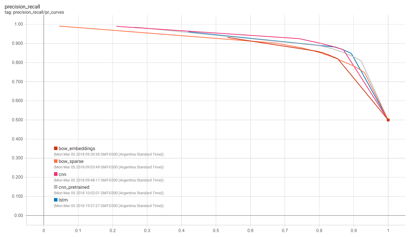
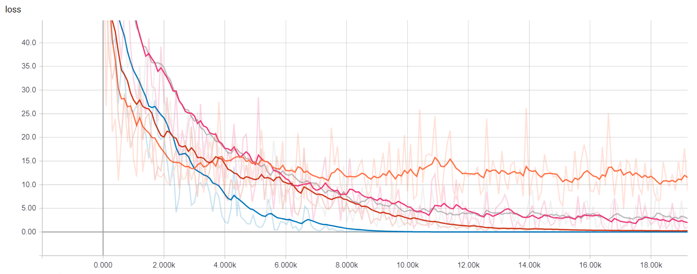
We can visualize many metrics collected while training and testing, including the loss function values of each model at each training step, and the precision-recall curves. This is of course most useful to select which model works best for our use-case as well as how to choose classification thresholds.
### Getting Predictions
To get predictions on new sentences we can use the `predict` method in the `Estimator` instances, which will load the latest checkpoint for each model and evaluate on the unseen examples. But before passing the data into the model we have to clean up, tokenize and map each token to the corresponding index, as shown here.
It's worth noting that the checkpoint itelf is not enough to make predictions since the actual code used to build the estimator is necessary as well, in order to map the saved weights into the corresponding tensors, so it's a good practice associate saved checkpoints with the branch of code with which they were created.
If your are interested in exporting the models to disk in a fully recoverable way you might want to look into the [SavedModel](https://www.tensorflow.org/programmers_guide/saved_model#using_savedmodel_with_estimators) class, specially useful for serving your model through an API using [TensorFlow Serving](https://github.com/tensorflow/serving).
"""
def text_to_index(sentence):
# Remove punctuation characters except for the apostrophe
translator = str.maketrans('', '', string.punctuation.replace("'", ''))
tokens = sentence.translate(translator).lower().split()
return np.array([1] + [word_index[t] + index_offset if t in word_index else 2 for t in tokens])
def print_predictions(sentences):
indexes = [text_to_index(sentence) for sentence in sentences]
x = sequence.pad_sequences(indexes,
maxlen=sentence_size,
padding='post',
value=0)
length = np.array([min(len(x), sentence_size) for x in indexes])
predict_input_fn = tf.estimator.inputs.numpy_input_fn(x={"x": x, "len": length}, shuffle=False)
predictions = {}
for path, classifier in all_classifiers.items():
predictions[path] = [p['logistic'][0] for p in classifier.predict(input_fn=predict_input_fn)]
for idx, sentence in enumerate(sentences):
print(sentence)
for path in all_classifiers:
print("\t{} {}".format(path, predictions[path][idx]))
print_predictions([
'I really liked the movie!',
'Hated every second of it...'])
"""### Other resources
In this notebook, we explored how to use estimators for text classification, in particular for the IMDB Reviews Dataset. We trained and visualized our own embeddings, as well as loaded pre-trained ones. We started from a simple baseline and made our way to convolutional neural networks and LSTMs.
For more details, be sure to check out:
* The complete [source code](https://github.com) for this blog post.
* A [Jupyter notebook](https://github.com) that can run locally, or on Colaboratory.
* The TensorFlow [Embedding](https://www.tensorflow.org/programmers_guide/embedding) guide.
* The TensorFlow [Vector Representation of Words](https://www.tensorflow.org/tutorials/word2vec) tutorial.
* The *NLTK* [Processing Raw Text](http://www.nltk.org/book/ch03.html) chapter on how to design langage pipelines.
In a following tutorial, we will show how to build a model using eager execution, work with out-of-memory datasets, train in Cloud ML, and deploy with TensorFlow Serving.
----------
*Thanks for reading! If you like you can find us online at [ruder.io](http://ruder.io/) and [@eisenjulian](https://twitter.com/eisenjulian). Send our way all your feedback and questions.*
"""