A simulation and set of configurations for calculating and exploring online search relevance metrics.
For a high-level introduction, please see the accompanying blog post, Analyzing online search relevance metrics with the Elastic Stack.
- Online Search Relevance Metrics
To run the simulation, you will first need:
- Elasticsearch and Kibana 7.7+ **
- Cloud Elasticsearch Service (free trials available)
- Local installations
make- Python 3.7+ (try pyenv to manage multiple Python versions)
virtualenv(installed withpip install virtualenv)
** Instructions and code have been tested on versions: 7.7.0, 7.8.0. Instructions reference Kibana and Cloud pages as of June 2020.
Use the Makefile for all setup, building, testing, etc. Common commands (and targets) are:
make init: install project dependencies (from requirements.txt)make clean: cleanup environmentmake test: run testsmake jupyter: run Jupyter Lab (notebooks)
Most operations are performed using scripts in the bin directory. Use -h or --help on the commands to explore their functionality and arguments.
To simulate and index events then run all transforms, use the bin/simulate script.
bin/simulate elasticsearchThe simulation will ensure that the right configurations in Elasticsearch are setup. You can also alter dimensions of the simulation such as the number of users. For example:
bin/simulate --num-users 1000 elasticsearchIf you are running a Cloud Elasticsearch Service instance you can set the Elasticsearch endpoint in simulate. To find the Elasticsearch endpoint, open your deployments, select a deployment, then under "Applications" you will find a link beside Elasticsearch to "Copy endpoint". Now use the url option to set the endpoint URL for your instance. Since security is enabled, you will need to also add the username and password in the URL. For example, the user elastic with password changeme can be set as follows:
bin/simulate elasticsearch --url https://elastic:changeme@YYY.us-central1.gcp.cloud.es.io:9243Use the -h or --help arguments to explore more functionality and arguments.
To recreate the visualisations in Kibana, you need to first make sure you have data in your Elasticsearch instance using the above simulate command. Then you just need to run kibana to create the dashboard, index pattern and visualizations.
bin/kibanaAs with simulate, if you are running on Cloud, ensure that your credentials are set and the correct Kibana URL is used (don't use the Elasticsearch URL!). You can find your Kibana endpoint just below where you found the Elasticsearch endpoint, and your credentials should be the same as with Elasticsearch.
bin/kibana --url https://elastic:changeme@YYY.us-central1.gcp.cloud.es.io:9243You're all set! Have a look at the Dashboard and Visualizations pages now and you should see a large set of ready-made visualizations. Make sure that your time range is set to the entire day of 15 Nov 2019 UTC.
In the blog post, we cover the motivation, set some context and outline the high-level approach to collecting and exploring online search relevance metrics in the stack. The remainder of this README contains implementation details which, should you want to implement the approach yourself, provide you will everything you need to get up-and-running fast!
The first thing to setup is the index in Elasticsearch that will store the user behaviour events: query, page and click. To describe the schema we'll be using the Elastic Common Schema (ECS). ECS is a good fit for this use-case since it already describes a large set of common attributes for events. We can reuse attributes like basic categorical, timestamp and user information, instead of having to describe them ourselves. When using ECS, we also get some features for free in Kibana such as the Logs and Maps apps.
We don't need all of the ECS field sets, so we'll stick to a subset for now. If you have more ECS fields that you can or want to use, you are welcome to do so. A snippet from the schema shows some of the ECS fields we need.
{
    "@timestamp": {
      "type": "date"
    },
    "ecs": {
      "properties": {
        "version": {
          "ignore_above": 1024,
          "type": "keyword"
        }
      }
    },
    "event": {
      "properties": {
        "action": {
          "ignore_above": 1024,
          "type": "keyword"
        },
        "dataset": {
          "ignore_above": 1024,
          "type": "keyword"
        },
        "duration": {
          "type": "long"
        },
        "id": {
          "ignore_above": 1024,
          "type": "keyword"
        }
      }
    }
}
Some attributes of our events are not described in ECS, but we can easily extend ECS with custom fields for our specific solution. Here's some fields that we will need. The purpose of each field is described in the custom field set.
{
  "SearchMetrics": {
    "properties": {
      "click": {
        "properties": {
          "result": {
            "properties": {
              "id": {
                "ignore_above": 1024,
                "type": "keyword"
              },
              "rank": {
                "type": "long"
              },
              "reciprocal_rank": {
                "type": "float"
              }
            }
          }
        }
      },
      "query": {
        "properties": {
          "id": {
            "ignore_above": 1024,
            "type": "keyword"
          },
          "page": {
            "type": "long"
          },
          "value": {
            "ignore_above": 4096,
            "type": "keyword"
          }
        }
      },
      "results": {
        "properties": {
          "ids": {
            "ignore_above": 1024,
            "type": "keyword"
          },
          "size": {
            "type": "long"
          },
          "total": {
            "type": "long"
          }
        }
      }
    }
  }
}
With the extended ECS schema we can create the event index ecs-search-metrics. Make sure that you configure the index settings appropriate for your environment as the settings that are generated are not for production purposes (e.g. number of shards and replicas).
Have a look at the simulation's ecs-search-metrics index configuration for a complete example of this step: config/indices/ecs-search-metrics.json
(Optional reading! Feel free to skip this if you are OK using the ECS schema already generated in this project.)
Given a subset of ECS fields that we need, plus custom fields that we want to add, we can generate an ECS compatible schema from a clone of the ECS repository. We want to stick to a specific commit in the HEAD of master for now, so we also checkout a specific commit.
git clone git@github.com:elastic/ecs.git && \
  cd ecs && \
  git checkout 994f7777b53ba31fe55dffd0667b347fb8afdfee
Now run the generator.py script to generate a new schema. This will use the configuration in config/ecs to define which ECS fields to use and the definition of custom fields.
Please make to set the SIM_DIR variable before running this to reference this codebase on your local drive.
export SIM_DIR=...
echo $SIM_DIR
make ve && \
build/ve/bin/python scripts/generator.py \
--ref v1.5.0 \
--subset $SIM_DIR/config/ecs/subset.yml \
--include $SIM_DIR/config/ecs/custom \
--out generated_customAfter generating the custom schema, you can find it in generated_custom/generated/elasticsearch/7/template.json. This will have to be changed again, manually, to set the index settings appropriate for the simulation. The easiest thing to do is just copy the properties of the mappings and replace that in the existing schema. All the index settings don't need to be copied.
The heart of calculating per-query metrics is in this step. Once you have events indexed in ecs-search-metrics, you can apply a transform to group events by their search query ID and calculate per-query metrics. This step requires three components: a transform, an ingest pipeline, and an output index.
As mentioned above, the transform is where we define the group-by strategy, as well as the basic aggregations we want to do on our events in each group. This includes any basic counting of events like total clicks, as well as descriptive statistics like the average number of clicks, etc.
Here's a snippet of the transform configuration showing some of the calculations performed on click events.
{
    "metrics.clicks": {
      "filter": { "term": { "event.action": "SearchMetrics.click" } },
      "aggregations": {
        "count": { "value_count": { "field": "event.id" } },
        "count_at_3": { "filter": { "range": { "SearchMetrics.click.result.rank": { "lte": 3 } } } },
        "max_reciprocal_rank": { "max": { "field": "SearchMetrics.click.result.reciprocal_rank" } },
        "mean_reciprocal_rank": { "avg": { "field": "SearchMetrics.click.result.reciprocal_rank" } },
        "first_click_time": { "min": { "field": "@timestamp" } },
        "last_click_time": { "max": { "field": "@timestamp" } }
      }
    }
}
The transform can be set up as either a continuous or batch transform. Continuous transforms are necessary when you want to calculate metrics on an ongoing basis from events that are being ingested on a continuous basis (e.g. in real time or hourly batches from an external source). Batch transforms can be used for experimentation as they are only able to be run once (the simulation uses batch transforms).
The ingest pipeline is used to take documents from the transform and calculate additional metrics that are easier to calculate in two steps, rather than in a complicated script in the transform. For example, any metrics that require a comparison between the original query event and the statistics from the transform group are best performed this way, such as time to first click which needs to find the difference between the query event and the first click event.
In the transform, we calculate the minimum click timestamp:
{
    "metrics.clicks": {
      "filter": { "term": { "event.action": "SearchMetrics.click" } },
      "aggregations": {
        "first_click_time": { "min": { "field": "@timestamp" } }
      }
    }
}
In the pipeline, we take the difference between the query and the minimum click timestamp to find the time to first click:
{
  "script": {
    "source": "ctx.metrics.clicks.time_to_first_click = ChronoUnit.MILLIS.between(ZonedDateTime.parse(ctx.query_event['@timestamp']), ZonedDateTime.parse(ctx.metrics.clicks.first_click_time))",
    "if": "ctx.metrics.clicks.first_click_time != null"
  }
}What comes out of the ingest pipeline is now ready to be stored in an index that will be our primary metrics index. We're giving it the super creative yet transparent name of ecs-search-metrics_transform_queryid (also matches the transform name) and it will contain all of the per-query documents that describe the original query event plus the metrics we calculated in the previous steps.
The schema for this index should include all the fields from the original query event, as well as the metrics we've calculated in the previous steps. Have a look at the schema for a complete example: config/indices/ecs-search-metrics_transform_queryid.json
Now that we have metrics calculated on a per-query basis and stored in an index, we can use various methods of aggregation to calculate metrics spanning over a period time and multiple users.
Let's start with the simplest way of calculating and showing metrics by executing an Elasticsearch Query to do some simple counting. There's no time bucketing, user filtering or aggregating — we'll save those for the next steps! For our CTR@3 example, we just need to find the two components of calculating CTR@3: the number of queries with clicks at 3 and the total number of queries with clicks.
The number of queries with results and clicks in any position:
POST /ecs-search-metrics_transform_queryid/_search?size=0
{
  "query": {
    "bool": {
      "must": [
        {
          "range": {
            "query_event.SearchMetrics.results.size": {
              "gt": 0
            }
          }
        },
        {
          "range": {
            "metrics.clicks.count": {
              "gt": 0
            }
          }
        }
      ]
    }
  }
}
The number of queries with results and clicks at 3:
POST /ecs-search-metrics_transform_queryid/_search?size=0
{
  "query": {
    "bool": {
      "must": [
        {
          "range": {
            "query_event.SearchMetrics.results.size": {
              "gt": 0
            }
          }
        },
        {
          "term": {
            "metrics.clicks.exist_at_3": true
          }
        }
      ]
    }
  }
}
Dividing the former by the latter gives us CTR@3, simple as that.
Some of the metrics we calculated per-query are even simpler to aggregate into single metrics. Take for example the time to first click. If we want to get a high-level understanding of the time it takes for users to click on the first result after executing the query, we simply take the average over a timeframe. If we want to include all of time, we can use the following average aggregation.
POST /ecs-search-metrics_transform_queryid/_search?size=0
{
  "aggs": {
    "avg_time_to_first_click": {
      "avg": {
        "field": "metrics.clicks.time_to_first_click"
      }
    }
  }
}
Returns:
{
  "took" : 4,
  "timed_out" : false,
  "_shards" : { ... },
  "hits" : { ... },
  "aggregations" : {
    "avg_time_to_first_click" : {
      "value" : 21222.222222222223
    }
  }
}
The same applies to any other per-query metric that we want to aggregate to a higher level. Typically they are just averages over a time period, but you can also explore other descriptive statistics such as variance, median, or extreme values such as 90th percentile. Check out the extended stats aggregation as a way to collect a set of descriptive statistics for a field.
POST /ecs-search-metrics_transform_queryid/_search?size=0
{
  "aggs": {
    "descriptive_stats": {
      "extended_stats": {
        "field": "metrics.clicks.time_to_first_click"
      }
    }
  }
}
Returns:
{
  "took" : 2,
  "timed_out" : false,
  "_shards" : { ... },
  "hits" : { ... },
  "aggregations" : {
    "descriptive_stats" : {
      "count" : 27,
      "min" : 3000.0,
      "max" : 49000.0,
      "avg" : 21222.222222222223,
      "sum" : 573000.0,
      "sum_of_squares" : 1.7223E10,
      "variance" : 1.8750617283950615E8,
      "std_deviation" : 13693.289336003463,
      "std_deviation_bounds" : {
        "upper" : 48608.80089422915,
        "lower" : -6164.356449784704
      }
    }
  }
}
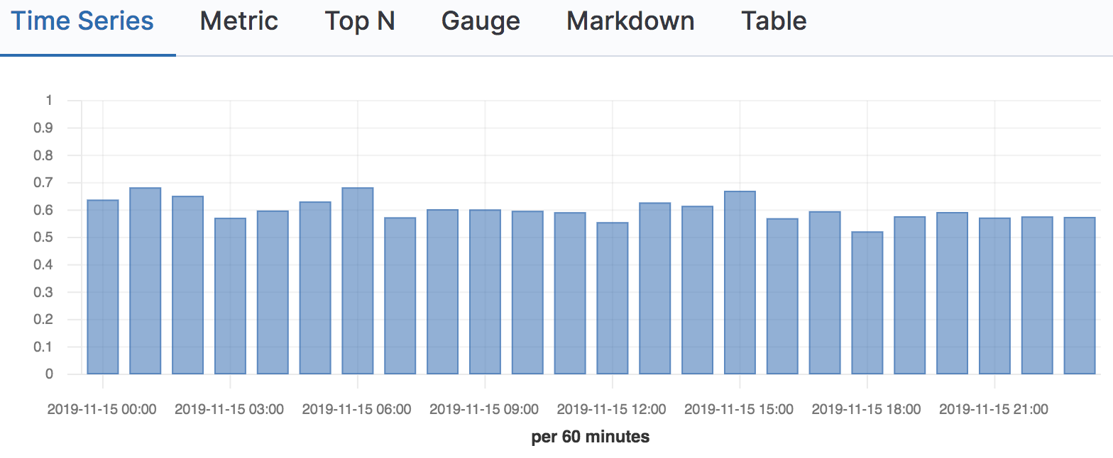
Now that we've seen some examples of calculating aggregate metrics directly with the Elasticsearch Query DSL, we know that we can use Kibana to visualize metrics and show more useful metrics that are bucketed by time. For example, plotting our CTR@3 metric can be achieved using a simple TSVB time series chart, bucketing out metrics every hour:
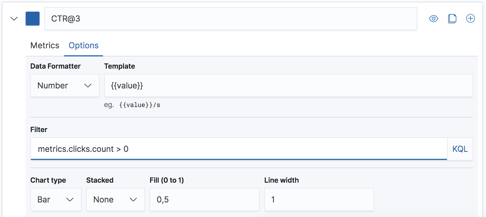
When we configure this time series chart for CTR@3 we only want to include queries that have clicks, so we'll set a filter on this time series using the KQL clause metrics.clicks.count > 0:

We'll use then a ratio filter to calculate ratio of the number of queries with clicks at 3 (KQL: metrics.clicks.exists_at_3 : true) over the number of queries with clicks in any position (KQL: *):
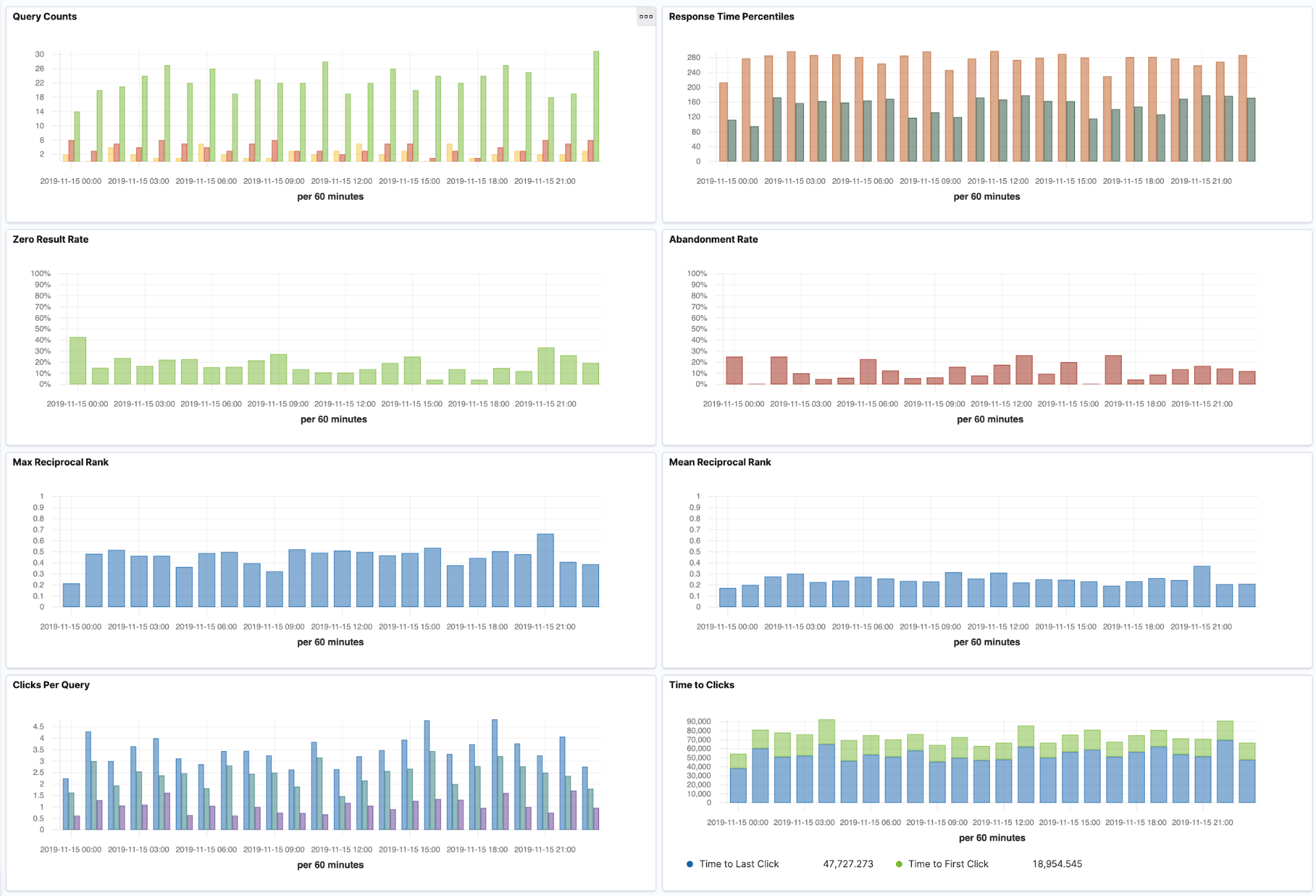
In this simulation project, we've created a large number of visualizations and a dashboard. These can be imported into a fresh Elasticsearch using Kibana's import saved objects feature. Instructions for this can be found above in the Kibana Visualizations section.
Sometimes we want to dig deeper into our datasets and metrics and using Kibana or the Elasticsearch Query DSL statements can be cumbersome or insufficient. Many Data Scientists and Analysts are more comfortable with using Python, Jupyter notebooks and Pandas to do this type of exploration. Using the eland library provides a Pandas interface to explore large datasets natively in Elasticsearch, by executing Elasticsearch queries and aggregations behind the scene. This allows you to explore all the metrics using a familiar interface.
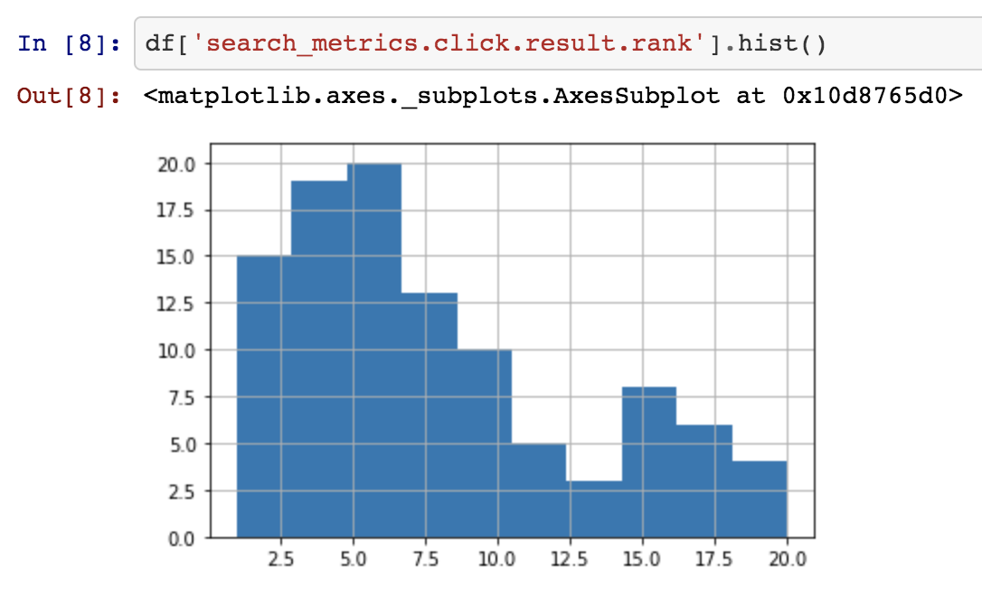
For a full example of calculating the same set of online search relevance metrics as in our Kibana example, check out the Jupyter notebook.