Authors
Change Log
Introduction
ExPRES
Connecting to ExPRES
ExPRES UI
SILFE
Connecting to SILFE
Datatree window
Plot Window
References
S. L. G. Hess
sebastien.hess@onera.fr
| Version | Name | Note |
|---|---|---|
| 1 | Keyuan Yin | First converted from this site |
ExPRES (Exoplanetary and Planetary Radio Emission Simulator) simulatea the planetary radio emissions related to auroral processes. It generates mainly synthetic dynamic spectra of planetary radio emissions. Its use and part of its code are described in section 2.
SILFE (Spectral Information from Low Frequency Emissions) displays the dynamic spectra from several sources, either observational (CASSINI, Nançay,...) or numerical (ExPRES). Its allows a simpler analysis and co mparison of all these sources. It is based on the IVAO VOTABLE standard for the data and on the IMPEx (SPASE extension) standard for the metadata.
The ExPRES online tool address is (as of Sept. 2014) : http://typhon.obspm.fr/maser/serpe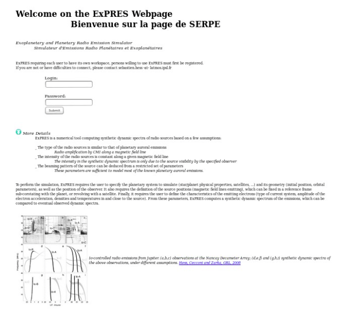
Figure 1: Font page of the ExPRES website
The front page gives a short description of the tool capabilities and invites the user to connect.
The connection necessitates a registration. The ExPRES tool is intended to be freely accessible to all users. However, as the actual software is run on the server and stores data on the server disk, an account needs to be created.
Once the login and password entered and submitted, you should be redirected to the ExPRES main page.
Main page layout
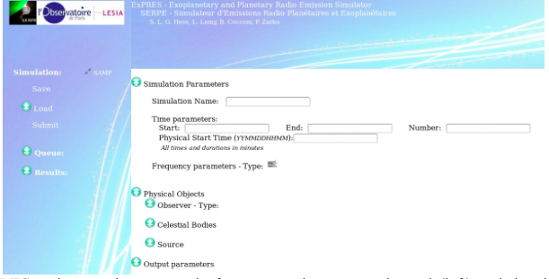
The ExPRES main page is composed of two parts the command panel (left) and the simulation setup panel (right).
Command panel
Its main purpose is to permits the user to manage simulation files (Load, save, delete,...) and the simulation runs (submit, follow, get results).
The simulation whose parameters are currently on the right simulation panel can be saved by clicking on Save and the simulation can be run by clicking on Submit.
The saved simulations can be displayed by clicking on the expand button Load. Then, a simulation can be loaded by clicking on the simulation name.
The queue can be viewed by clicking on the expand button Queue. Simulations can be either Running or Waiting.
The results can be accessed by clicking on the expand button Results. Then the data can be viewed by clicking on their name. The XML outputs, which follows the IVOA VOTable standard can be shared with third-party VO applications though the SAMP protocol by clicking on the icon. This can be used to display the results in SILFE.
To use the SAMP capabilities, it is necessary to connect to a SAMP hub by clicking on the SAMP icon. It can be disconnected by clicking at the same location on the icon. If no SAMP hub is running, you will be asked whether you want to run one from the astrojs@github repository.
Simulation Setup panel
General parameters
The general parameters cover the time and frequency domain covered by the simulation and allow to give a name to it.

The time settings are limited to the times at which the simulation starts and ends (in minutes, like all times and durations in ExPRES) and the number of time steps.
It is also possible to define a physical “zero” time by providing a date. This date is particularly used for the generation of the VOTable outputs, but are also used for ephemeris.
Frequency parameters are of three types that can be selected in a list. The linear and logarithmic scales are defined by minimum and maximum frequencies and the number of frequencies to simulate. Predefined frequencies also exist that corresponds to known instruments they can be selected by .
Observer
There are three types of observers : fixed ones whose position in the simulation reference frame does not vary ; orbiters which moves in the simulation reference frame, orbiting around a celestial body ; predefined observers which represent known mission around celestial bodies. To select the
type of observer, select it in the Type list (click o n  ).
In any cases, it is necessary to define the celestial body which serves as reference for the position of the observer. Open the parent list (click on  ) and select the reference celestial body.
(  Notes : 1- The selection is not updated, so if the celestial body is deleted or its name changed, the parent must be manually updated or the simulation will not run. 2- Obviously, at least one celestial body must be created before associating the observer to a body.).
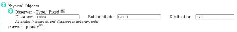
Fixed observer are parametrized by their distance to the reference body, their sublongitude and their declination (in the reference body reference frame and at initialization time).
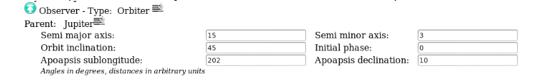
Orbiter orbits are defined by their semi-major and semi-minor axis, the apoapsis sublongitude and declination (in the reference body reference frame and at initialization time) and the inclination of the orbit plane around the semi-major axis.) Finally, the orbiter position requires the definition of its initial phase on the orbit (0deg. is at the apoapsis position).
(  Tips : The trajectories of all objects can be checked by using the 3D movie output).
Predefined types corresponds to the orbits of some missions whose ephemeris are provided by the AMDA tool of the French Plasma Physics Center (CDPP -).
Celestial bodies
Two types of celestial bodies can be included in the simulations, fixed bodies (at least one needed) and orbiting bodies (which can orbit both fixed and orbiting bodies).

Bodies can be created using the icon in the  celestial bodies section (expend by clicking on ).
They can be deleted by clicking on the  icon in front of their name.
The parameters of the celestial body can be set/modified by expending the section (click on ).
The body must be given a name. Each object must be given a different name as they are internally referred by it in ExPRES.
The body radius must be indicated. Contrary to the other quantities in ExPRES, the unit of the lengths and distances are arbitrary. However, the units must be consistent through a simulation parameter set.
The body's period and the Keplerian period at the body's surface must be defined in minutes.
The orientation of the body relative to the simulation reference frame is given by the sublongitude of the x-axis at the simulation start.
The model of the body's magnetic field can be selected (click on  ).
User defined dipolar magnetic field can be set by clicking on “User defined Dipole (No CS)”. The parameters of the dipole must be set by filling the field that appear when clicking on the  icon. The user is asked the dipole moment (in Gauss/Planet radii3), the tilt of the magnetic field (tilted toward in the body reference meridian) and the offset of the dipole relative to the planet center.
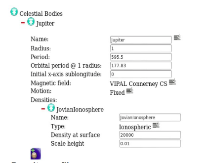
Density profiles
To each celestial body can be associated several (plasma) density profiles. Four types of density models exist : ionospheric (exponential decrease versus distance), stellar (decreases as the distance squared), disk (exponential decrease with altitude relative to equatorial plane and distance), and torus, (exponential decrease from the center of a torus of given radius).
These profiles can be set by clicking on the  icon, and deleted by clicking on the  icon.
The profiles must be given a unique name and the profile type can be selected in the profile list (click on  ). The profile parameter will be asked below.
Satellites
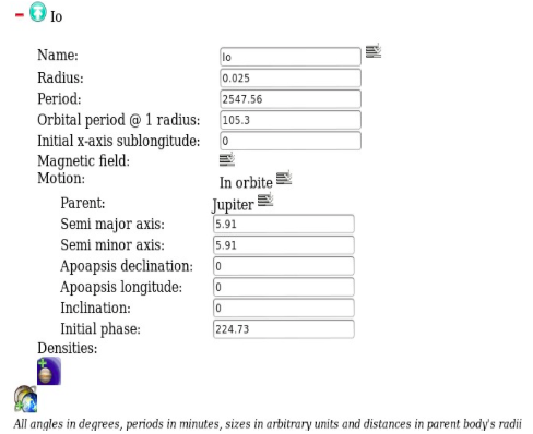
The body can be made orbiting another one by changing the Motion selection from Fixed to In orbite. In this case, the body's parent must be set by selecting a parent body in the list (click on).
(  Notes : 1- The selection is not updated, so if the celestial body is deleted or its name changed, the parent must be manually updated or the simulation will not run. 2- Obviously, the parent celestial body must be created before associating the it to a body.).
Satellite orbits are defined by their semi-major and semi-minor axis, the apoapsis sublongitude and declination (in the reference body reference frame and at initialization time) and the inclination of the orbit plane around the semi-major axis.) Finally, the orbiter position requires the definition of its initial phase on the orbit (0deg. is at the apoapsis position).
(  Tips : The trajectories of all objects can be checked by using the 3D movie output).
Sources
Radio sources can be added by expending the source section (click on the icon in front of the source section) and clicking on the  icon. Once created, they can be deleted by clicking on the icon.
They must be given a unique name.
Their parent body (body on which field lines the source is located) must be specified by clicking on the
( Notes : 1- The selection is not updated, so if the celestial body is deleted or its name changed, the parent must be manually updated or the simulation will not run. 2- Obviously, the parent celestial body must be created before associating the it to a body.).
The source parameters (type of current, electron energies and temperatures, ...), that are defined in a paper (), must be specified. The steady-state current implies an emission by a shell-distribution obtained by the parallel acceleration (energy increase ) of a bi-Maxwellian distribution (defined by the core and halo temperatures).
The hemisphere(s) is which the source is located can be selected using the checkboxes. Then, the
position and motion of the magnetic field line on which the source is located must be selected.
The emission pattern is a deformed hollow cone (deformation due to refraction). The width of the conical sheet is given by the “Beam width” field.
It can either be attached to a satellite, fixed in equatorial L-Shell or in surface latitude. The selection is made in the “Active field line” list (click on  )
(  Notes :In any cases, the possibilities for magnetic field line positions are limited by the fact that they must be pre-computed – with a precision or step of 1degree in longitude and latitude or distance. If you needs exceed the existing possiblities please contact the maintenance contact person. At this time Dr. B. Cecconi: baptiste.cecconi@obspm.fr).
Attached to a satellite
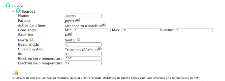
For source attached to a satellite, the satellite must be selected in the Satellite list (click on  ).
The motion of the field line will be that of the satellite. A set of lead angles can be defined be giving a minimum and maximum lead angles, and the number of active field lines.
Fixed in L-Shell
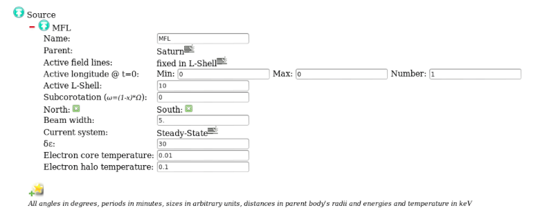
For sources fixed in L-Shell, the field line motion is in corotation by default, but a subcorotation rate can be set in the “Subcorotation” field (0 = rigid corotation, 1 = no rotation at all).
The L-Shell of the active field lines can be set in the “Active L-shell” field, and the longitudinal position of the active magnetic field lines can be set by providing the minimum and maximum longitudes of the active field lines and the number of active field lines..
Fixed in latitude
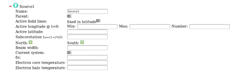
For sources fixed in magnetic latitude, the field line motion is in corotation by default, but a subcorotation rate can be set in the “Subcorotation” field (0 = rigid corotation, 1 = no rotation at all).
The latitude of the active field lines can be set in the “Active latitude” field, and the longitudinal position of the active magnetic field lines can be set by providing the minimum and maximum longitudes of the active field lines and the number of active field lines..
Outputs
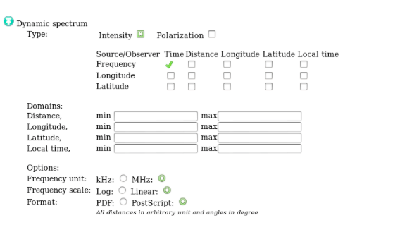
Dynamic spectra
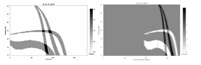
ExPRES standard outputs are dynamic spectra (intensity in the time-frequency domain). But ExPRES can also display the intensity as a function of observer or source longitude, source latitude, or local time or observer distance. This can be managed by selecting the corresponding checkboxes in the type section. The longitude/latitude/local time/distance ranges to be display must be specified in the corresponding fields.
ExPRES can also display the polarization (positive for northern sources, negative for southern ones) in the same manner. This can be done be selecting the polarization checkbox.
The frequency axis unit, the output format, and the frequency scale can be chosen using the Options checkboxes.
2D movies
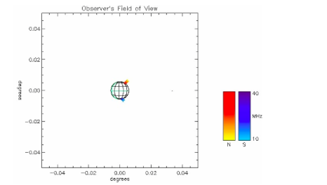
ExPRES can also display the position of the observed sources in the field of view of the instrument. This is done by adding a 2D movie in the simulation (click on  2D movie).
Then, it is needed to specify the Field of view opening in degrees, that is the extent of the part of the sky to be displayed. It is also needed to specify the subcycling for the movie, that is the number of simulation time steps between to successive pictures.
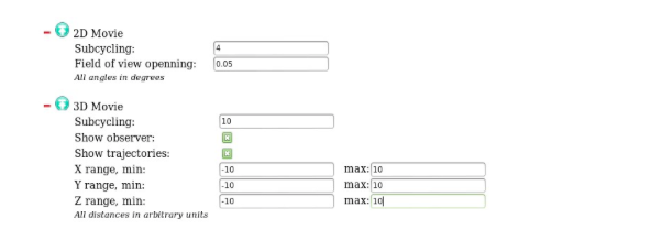
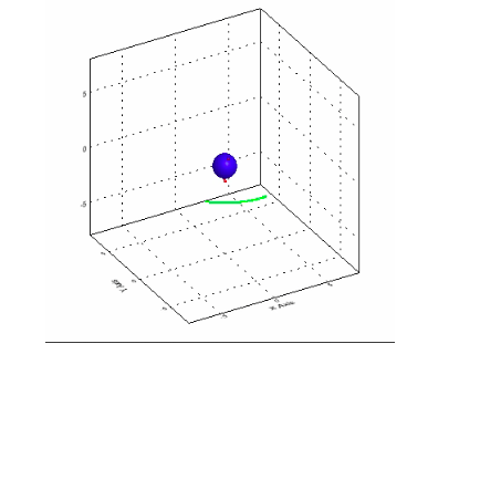
3D movies
ExPRES can also display the celestial bodies and sources position in 3D. This is done by adding a 3D movie in the simulation (click on  3D movie).
The trajectories of the satellites and observers can be displayed by checking the corresponding checkboxes.

Then, it is needed to specify the spatial domain to be displayed. It is also needed to specify the subcycling for the movie, that is the number of simulation time steps between to successive pictures.
The SILFE online tool address is (as of Sept. 2014) : http://typhon.obspm.fr/maser/SILFE. The SILFE tool does not use user-specific workspaces and thus does not require login for use.
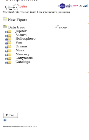
Once connected to SILFE a popup window should appear which displays the data tree from the REDCAT repository.
Components
The datatree window is composed of the  icon which permits to start a new plot window (there is no limits on the number of plot windows simultaneously opened). It also has an icon to start a connection to the SAMP services . To use the SAMP capabilities, it is necessary to connect to a SAMP hub by clicking on the SAMP icon  . It can be disconnected by clicking at the same location on the  icon. If no SAMP hub is running, you will be asked whether you want to run one from the astrojs@github repository.
The main component of the datatree window is obviously the datatree. It displays all the data referenced by the Radio Emission Databases CATalog (REDCAT) as a tree. The data are ordered by target (e.g. celestial body), by instruments or simulation code (within a single database), by the type of data and by datasets. Datasets (indicated by the  icon) are the elements that can be selected for display.
Fields
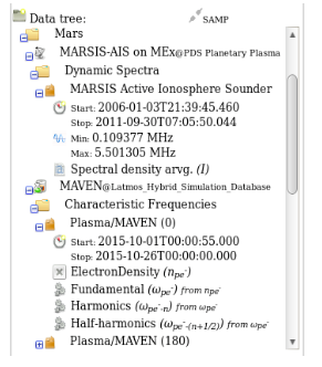
Observational datasets are marked with the  icon at the instrument level, and simulation/model with the  icon. When a dataset is selected, it displays the dataset time span and frequency range. It also shows (with the  icon) all of the fields contained in the dataset that can be visualized (datasets may contain more data than displayed but that cannot be displayed by SILFE). However, some datasets which serves as source from derived fields that can be displayed by SILFE may appear, with the  icon.
Further information about the dataset can be obtained by performing a right click on the dataset name and by clicking on the  icon.
Physical content of a field
SILFE may auto-detect the physical content of each field (from the UCD is specified in the data file), in which case it is displayed in parenthesis after the field name:
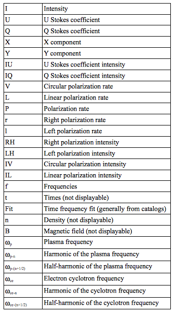
When SILFE recognizes several physical contents in the same dataset, in generates new fields from those. These derived fields are marked with the  icon. The fields from which they are computed are indicated in the parenthesis.
User's data
User can import its own data from SAMP. These data must be at the VOTable format. These data appear in the User top folder.
Catalog
Catalogs of radio emissions are also available in SILFE. Catalogs can be accessed by performing a right click on the dataset name. Then the catalog is accessed by clicking on the  icon.
Some of the catalog contain fits of the data. And can be displayed in the plot window as any dynamic spectrum.
To open a plot window, click on the icon  in the datatree window as shown of the figure on the right.
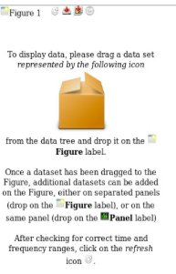
Plotting a field
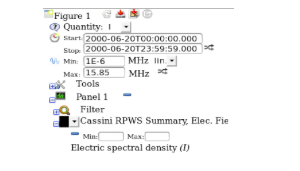
To plot a field in the plot window, select the corresponding dataset in the datatree and drag it (by keeping the left mouse button pressed) over the “ Figure X” label. A horizontal bar should appear below the label. Then drop it (release the mouse button). The detail of the field will appear on the left side of the window.
At this stage, the plot time span (start and end time) are displayed and can be modified, as well as the frequency range (minimum value, maximum value) and the frequency scale (Linear, Logarithmic, Altitudinal (prop. to f1/3)). These are global values which affects all datasets and panels when modified. This can be switched to independent time span and/or frequency range by clicking on the  icon.
The quantity represents the physical quantity to plot. It will affect all the fields in all the plots.
When the dataset has been dropped, a new panel (Panel 1) has been created that contains the dataset. A panel represents a single plot: two datasets in the same panel are overplotted.
The color used to display the data of the dataset is shown in front of its name. It can be changed by clicking on the color. The detail of the dataset can be obtained by clicking on  . Then the dataset can be removed by clicking on the  icon. The min and max values to plot (in the dataset own unit) can be modified and the data field to be plotted is displayed. It can be changed by clicking on it and choosing the field in the list.
Then the field can be plotted by clicking on the refresh icon  at the top of the window.
Save and share
To save the data used to generate the plots, click on the  icon. The data will be saved as a VOTable. By clicking on the  icon, the VOTable will be shared with other VO tools via the SAMP protocol, if SILFE is connected to SAMP. Click on the  icon to save the picture of the plot as a PNG.
Plotting in another panel
To plot another field on the another panel, choose the dataset to plot in the datatree, drag it over the Figure label until a horizontal line appear under it (exactly as for the first field) and drop it (release the mouse button).
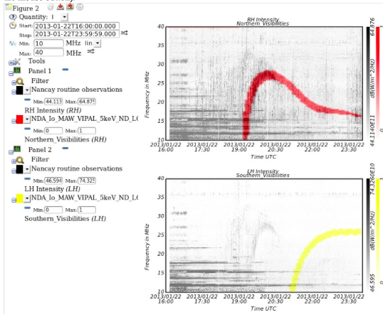
Overplotting a second field
To plot another field on the same panel, choose the dataset to overplot in the datatree, drag it over the targeted panel until a horizontal line appear under the panel label and drop it.(release the mouse button).
Please refer this tutorial to original version on this site