In this example we will use data available from epn1.epn-vespa.jacobs-university.de
The tutorial is covered by the following YouTube video:
This tutorial will demonstrate how to:
-
Install plugins we have developed.
-
Browse WMS layers exposed on our server and load them as basemap in QGIS.
-
Run complex geospatial queries using ADQL on DaCHS and load it to QGIS using our plugin.
-
Load previews of CRISM coverages onto the map.
-
Access spectra of individual pixels on CRISM coverages of interest and broadcast this data to VO spectroscopy applications such as CASSIS.
The following python modules are required:
- PyQt4
- os
- qgis
- astropy
- shapefile
- numpy
- tempfile
- geojson
- urllib
- threading
- time
https://github.com/epn-vespa/VO_QGIS_plugin/archive/v0.2.zip
The QGIS plugin directory should then look like:
~/.qgis2/python/plugins
├── GAVOImage
├── polyToAladin
└── VESPA

- Opening epn1.epn-vespa.jacobs-university.de, clicking on TAP, than TapHandle or
- Going directly to http://saada.unistra.fr/taphandle/?url=http://epn1.epn-vespa.jacobs-university.de/tap


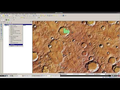
In our case it's


You should now have a basemap displayed on your Canvas.
The data aquisition process consists of 4 fundamental steps: 0. Data mining / querying
- Starting SAMP Hub
- Starting SAMP Clinet
- Transfering data via SAMP
The workflow follows as such:

Suppose we are interested in CRISM coverages from sensor L that cover craters of diameter between 50 and 80 km. We can do this with an ADQL query. Simply paste this request into browser:
http://epn1.epn-vespa.jacobs-university.de/__system__/adql/query/form?__nevow_form__=genForm&
query=select cra.granule_uid, cri.*, cra.diameter, cra.feature_name, cra.crater_morphology_3 FROM (select * from mars_craters.epn_core as cra2 where cra2.diameter > 50 and  cra2.diameter < 80) as cra INNER JOIN (select * from crism.epn_core as cri2 where cri2.sensor_id='L') as cri  ON (1=INTERSECTS(
cri.s_region,
cra.s_region
))&_TIMEOUT=200&_FORMAT=HTML&submit=Go

Detailed instructions on what ADQL is and how to use it are beyond the scope of this tutorial and can be found on the bottom of that webpage, or on: http://epn1.epn-vespa.jacobs-university.de/__system__/adql/query/info


2.3.2 Click again on "Send via SAMP" and wait for table to download. Once it is added to the Layers Panel, click on "Connect/Disconnect", press OK (this will close the client), then close SAMP HUB as well.
Your table will now appear in the Layers Panel


You should now be able to see the preview image over the polygon.

By using "Identify tool" on the corresponding polygon you can learn more about the crater:

We can use the data in the table to examine spectra of a particular location on Mars. Furthermore, this data can then be sent via SAMP to VO spectroscopy tools, such as CASSIS.


Open Aladin web start: aladin.u-strasbg.fr/java/aladin.jnlp
On the main menu click "File" => "Open URL"

Add HiPS :
http://epn1.epn-vespa.jacobs-university.de:8080/marsmola/Mars-ELATLON-ICRS.hpx
Click submit.

5.1 In QGIS select several polygons from a table recieved via SAMP and click on the polyToAladin plugin button

Polygons will now appear in Aladin
