Using continuous external regressors #484
Comments
|
For standardization: The future dataframe should have original, not-standardized values, and the forecasted values should also not be standardized. For predictions, Prophet will apply the same standardization offset and scale used in fitting. I have a few comments about the extra regressor fit.
We should add an example with a continuous regressor. The biggest challenge with a continuous regressor is exactly this second point: You need a good forecast of the regressor in order for it to be useful, which I think limits the applicability of continuous extra regressors. As for forcing trend = 0: That's an interesting question. You can set the number of changepoints to be 0, but will still then have a linear trend. There isn't a way right now to force no trend. |
|
Hi Ben, I am using continous external regressors as well, but I have an issue with seasonality being mistaken for impact of these regressors. Due to this I am receiving negative forecast. Is there a way to avoid this? Thanks, |
|
(The negative forecast is only ONE data point out of 52) Every mid-July now goes negative due to external regressor. |
|
@deniznoah can you post a plot of the forecast and of the forecast components so I can see what is going on? |
|
@bletham I have noticed it has something to do with the amount of data loaded in the external regressors. When I uploaded more promotions is corrected itself. I have one part I did not understand though. That is: I load my future external regressors in "future", and fit my model. After that when I check my "forecast" figure it appears to have different figures for external regressors. Is it forecasting my external regressors as well? I do not want the model to change the external regressors I put in. I hope this is not the case. Can you please help clarify?
|

|
|
|
Makes a lot of sense now. So i don't have to worry about it being different than the future value. Thanks for the great explanation! Another issue that I am facing is I would like to stop my forecasts from going "negative". Is there a way to automate linear vs. logistic growth? Also how would I determine a "cap" for logistic growth? All I care about is that my forecast does not go negative... |
|
If you set the growth to logistic then it will saturate at 0. You do then have to specify a cap - it could just be a really big value that you're sure your forecast should always be less than. There isn't yet a way to get the floor on the bottom (0) without having to specify a cap on top. This is on the todo list in #307, but I think we'll wait until #501 is done before doing that. One thing to note is that using logistic growth will force the trend to be positive, but the seasonality is added to that, and could still dip below 0. You'd have to just clip the forecasts at 0. Multiplicative seasonality would keep it positive, that will be out in the next version very soon. (You can test multiplicative seasonality in the v0.3 branch now if you'd like, see #254). |
|
I think this issue has been resolved but feel free to reopen if there are more questions. I'll add an example of a continuous extra regressor in the future. |
|
Using external regressors, in order to create a what if scenario, I may use the forecasted effect of every extra regressor? |
|
@dajerman yes, with the caveat that your forecast can only then be as good as the forecast for your extra regressor. For a "what-if" counterfactual evaluation, that seems quite reasonable. In general, if you are using a forecast in an extra regressor, the uncertainty in the extra regressor forecast will not be incorporated into the uncertainty estimates given by Prophet, which means that the Prophet uncertainty estimates will underestimate the true uncertainty. |
|
@bletham First of all, many thanks for this great package! I have a question regarding the uncertainty in the extra regressor forecast.
So basically 2 and 3 as pseudo code: # Draw 1000 samples from posterior predictive distribution of the regressor
pred_samp_regressor <- prophet::predictive_samples(m1, future1)
# For each of the 1000 samples predict y for the main model
forecast_samples <- list()
for (i in 1:1000) {
future2$extra_regressor_col <- pred_samp_regressor$yhat[,i]
forecast <- prophet::predict(m2, future2)
forecast_samples[[i]] <- forecast$yhat
}Would this make sense from your perspective? Thanks a lot! |
|
I think that's really close to what you'd want to do. This actually just came up in #1392 a few weeks ago, and this is the procedure I proposed there: #1392 (comment) The difference between what I proposed there and your procedure is whether we get If you use If you use Does that make sense? |
|
Makes perfect sense! Thanks a lot for the quick reply! |
I am struggling implementing continuous external regressors. According to the documentation this should be possible, however the documentation is currently lacking an example.
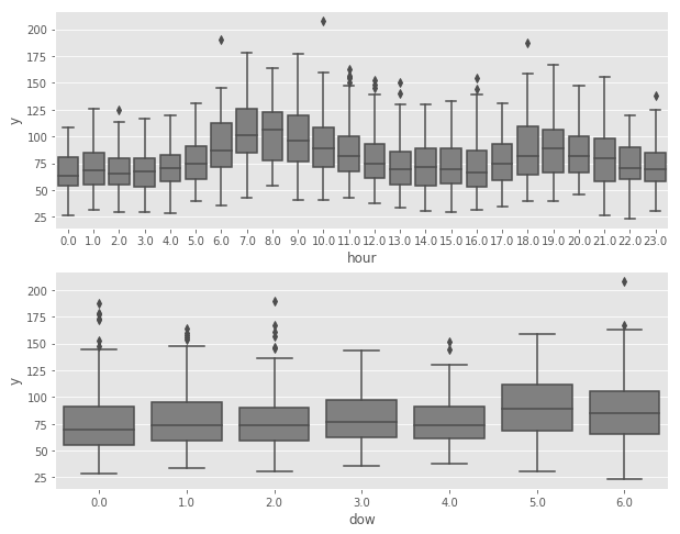
I am looking at a timeseries (thermal demand for a building = y), which shows a clear diurnal cycle (upper part of graph). In addition, there is also a weak weekly cycle (lower part of graph):
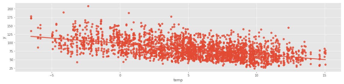
Furthermore, there is a clear dependency on the outside temperature:
First, I am creating a model adding the external regressor (= outside temperature) using
add_regressor.My understanding is, that internally the regressor is being normalized if called without an additional parameter (standardize=False).
Next, I am creating the forecast dataframe for the next 48hours, copy the historical temperature values as well as copy the temperature forecast:
--> do I need to copy the normalized (forecast) temperature values or the regular values?
Fitting the model without the additional regressor, I obtain a mean squared error of 0.0572
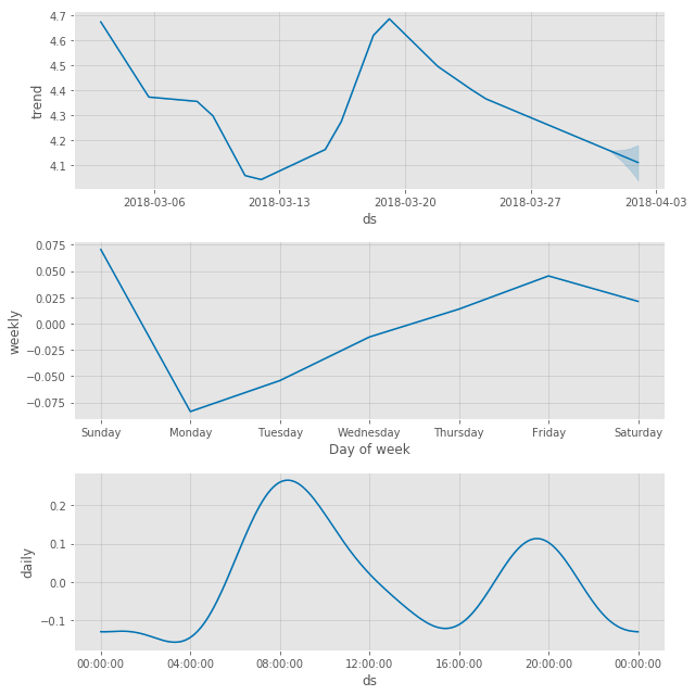
Including the additional regressor, the mean squared error is reduced, however only slightly: 0.056
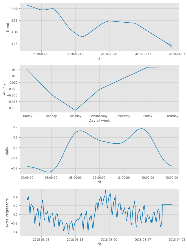
I am surprised that the outside temperature feature has such a low importance despite its clear causality and relation as shown above.
Am I doing something wrong using the external regressor feature?
Furthermore, is it possible to enforce the trend component = 0?
The text was updated successfully, but these errors were encountered: