1. Introduction
1.1. What is micompm?
1.2. Basic concepts
1.3. Available functions
2. The micompm workflow
2.1. Getting started
2.2. Data layout and data file format
2.3. Compare observations from two or more groups
2.4. Verify assumptions for the performed parametric tests
2.5. Multiple comparisons and different outputs
2.6. Visualization and publication quality tables
3. Tutorial
3.1. Loading simulation data
3.2. Comparing implementation outputs
3.3. Assessing distributional assumptions
3.4. Simultaneous comparisons of multiple outputs
4. Limitations
5. Unit tests
6. References
micompm [1] is a MATLAB/Octave port of the original micompr R [2] package for comparing multivariate samples associated with different groups. It uses principal component analysis (PCA) to convert multivariate observations into a set of linearly uncorrelated statistical measures, which are then compared using a number of statistical methods. This technique is independent of the distributional properties of samples and automatically selects features that best explain their differences, avoiding manual selection of specific points or summary statistics. The procedure is appropriate for comparing samples of time series, images, spectrometric measures or similar multivariate observations. It is aimed at researchers from all fields of science, although it requires some knowledge on design of experiments, statistical testing and multidimensional data analysis.
If you use micompm, please cite reference [1].
Given n observations (m-dimensional), PCA can be used to obtain their representation in the principal components (PCs) space (r-dimensional). PCs are ordered by decreasing variance, with the first PCs explaining most of the variance in the data. At this stage, PCA-reshaped observations associated with different groups can be compared using statistical methods. More specifically, hypothesis tests can be used to check if the sample projections on the PC space are drawn from populations with the same distribution. There are two possible lines of action:
- Apply a MANOVA test to the samples, where each observation has q-dimensions, corresponding to the first q PCs (dimensions) such that these explain a user-defined minimum percentage of variance.
- Apply a univariate test to observations in individual PCs. Possible tests include the t-test and the Mann-Whitney U test for comparing two samples, or ANOVA and Kruskal-Wallis test, which are the respective parametric and non-parametric versions for comparing more than two samples.
The MANOVA test yields a single p-value from the simultaneous comparison of observations along multiple PCs. An equally succinct answer can be obtained with a univariate test using the Bonferroni correction or a similar method for handling p-values from multiple comparisons.
Conclusions concerning whether samples are statistically similar can be drawn by analyzing the p-values produced by the statistical tests, which should be below the typical 1% or 5% thresholds when samples are significantly different. The scatter plot of the first two PC dimensions can also provide visual, although subjective feedback on sample similarity.
While the procedure is appropriate for comparing multivariate observations with highly correlated and similar scale dimensions, assessing the similarity of “systems” with multiple outputs of different scales is also possible. The simplest approach would be to apply the proposed method to samples of individual outputs, and analyze the results in a multiple comparison context. An alternative approach consists in concatenating, observation-wise, all outputs, centered and scaled to the same order of magnitude, thus reducing a “system” with k outputs to a “system” with one output. The proposed method would then be applied to samples composed of concatenated observations encompassing the existing outputs. This technique is described in detail in reference [3] in the context of comparing simulation outputs.
The typical micompm workflow is based on the following functions:
- grpoutputs - Load and group outputs from files containing multiple observations of the groups to be compared.
- cmpoutput - Compares output observations from two or more groups.
- micomp - Performs multiple independent comparisons of output observations.
- micomp_show - Generate tables and plots of model-independent comparison of observations.
- cmpassumptions - Verify the assumptions for parametric tests applied to the comparison of output observations.
Note that some of the statistical tests available in MATLAB and Octave, used in the cmpoutput and cmpassumptions functions, return slightly different p-values. micompm also provides and uses additional helper and 3rd party functions.
Clone or download micompm. Then, either: 1) launch MATLAB/Octave directly
from the micompm folder; or, 2) within MATLAB/Octave, cd into the
micompm folder and execute the startup script.
Note that micompm requires the MATLAB Statistics toolbox (when used with MATLAB) or the Octave statistics package (when used with Octave).
The basic data layout used in micompm consists of n x m matrices, each matrix representing an output, where n is the number of observations and m corresponds to the number of variables or dimensions. Individual observations in these matrices must be associated with a group. This association is expressed with a n-dimensional integer vector, where its i th value corresponds to the i th observation (row) of the output matrix. For example:
data =

    0.5341    0.6815    0.0190    0.5497   46.4804
    0.0900    3.3933    0.0495    8.5071   34.8334
    0.1117    2.4759    0.0148    5.6056   29.1395
    0.6523    0.0037    0.1980    5.6094   19.8188
    0.7032    6.0581    0.1055    1.5949   12.6425
    0.7911    4.2880    0.0959    3.4867   18.5939

groups =

    1     1     1     2     2     2
In this example, the data matrix contains six five-dimensional
observations. The groups vector specifies that the first three observations
(rows) are associated with group 1, while the last three belong to group 2.
The grpoutputs function loads and groups outputs from files containing observations of the groups to be compared. Each individual file represents an observation, and must be comprised of numerical data with m rows and g columns, where rows correspond to dimensions or variables and columns to different outputs. The grpoutputs function returns two variables: 1) a cell array containing g output matrices (n x m); and, 2) a n-dimensional integer vector defining the group each observation belongs to. In other words, grpoutputs returns data ready to be used in other micompm functions.
The cmpoutput function compares observations from two or more groups and is at the core of the micompm toolbox. Its prototype is as follows:
[npcs, p_mnv, p_par, p_npar, scores, varexp] = cmpoutput(ve, data, groups, summary)The first parameter, ve, specifies the percentage of variance which must be
explained by the principal components (PCs) compared in the MANOVA test. More
precisely, it determines the number of PCs used in the test. The second
parameter, data, is the n x m output matrix containing the data to be
compared, while the third parameter is the n-dimensional vector specifying
the groups to which the observations in data belong to. The last parameter,
summary, is optional and defines the number of PCs to show the p-values for
in the case of univariate tests. It can be set to 0 in order to completely
suppress the comparison summary. Besides printing this summary, cmpoutput
returns the following information:
npcs- Number of principal components which explainvepercentage of variance.p_mnv- P-value for the MANOVA test fornpcsprincipal components.p_par- Vector of p-values for the parametric test applied to groups along each principal component (t-test for 2 groups, ANOVA for more than 2 groups).p_npar- Vector of p-values for the non-parametric test applied to groups along each principal component (Mann-Whitney U test for 2 groups, Kruskal-Wallis test for more than 2 groups).scores- n x (n - 1) matrix containing projections of output data in the principal components space. Rows correspond to observations, columns to principal components.varexp- Percentage of variance explained by each principal component.
The cmpoutput function performs several statistical tests, including the
t-test or ANOVA (on each PC) and MANOVA (on the number of PCs that
explain ve percentage of variance). These tests are parametric, which means
they expect samples to be drawn from distributions with particular
characteristics, namely that: 1) samples are drawn from normally distributed
populations; and, 2) samples are drawn from populations with equal variances.
The cmpassumptions function performs additional tests that verify these
assumptions. It is invoked as follows:
[p_unorm, p_mnorm, p_uvar, p_mvar] = cmpassumptions(scores, groups, npcs, summary)The function accepts as arguments the PCA scores returned by cmpoutput,
the groups to which the observations in scores belong to, and the number of
PCs (for the multivariate comparison with MANOVA). The summary argument
plays a similar role to cmpoutput's equivalent. cmpassumptions returns
p-values for the assumptions tests, namely:
p_unorm- Matrix of p-values from Shapiro-Wilk's test of univariate normality. Rows correspond to groups, columns to PCs.p_mnorm- Vector of p-values from Royston's test of multivariate normality (onnpcs), one p-value per group.p_uvar- Vector of p-values from Bartlett's test of equality of variances, one p-value per PC.p_mvar- P-value from Box's M test of homogeneity of covariance matrices (onnpcs).
P-values smaller than the typical 0.05 or 0.01 thresholds may be considered statistically significant, casting doubt on the respective assumption. However, as discussed in reference [3], analysis of these these p-values is often not so clear-cut.
The micomp function performs multiple comparisons of different outputs, making use the functionality provided by grpoutputs and cmpoutput. It is invoked as follows:
c = micomp(nout, ccat, ve, varargin)The nout parameter specifies the number of outputs to compare, including an
optional concatenated output. The centering and scaling method for the optional
concatenated output is given in the ccat parameter (available options are
'center', 'auto', 'range', 'iqrange', 'vast', 'pareto' or 'level'); if ccat
is set to 0 or '', the concatenated output is not generated. The ve argument
defines the percentage of variance explained by the q principal components
(i.e. number of dimensions) used in the MANOVA test. The remaining arguments,
varargin, define the data and comparisons to be performed.
The micomp function returns a struct with several fields containing the results provided by cmpoutput for all comparisons and outputs.
Plots and publication quality tables summarizing the performed comparisons can be generated with the micomp_show function. The prototype of this function is simple:
[tbl, fids] = micomp_show(type, c, nout, ncomp)The first parameter, type, defines the type of output to generate. If set to
0, a LaTeX table is generated, while setting it to 1 yields a plain text table.
Setting type to 2 also produces a plain text table, but additionally
generates a number of plots summarizing the performed comparisons. The second
parameter, c, is the struct returned by the micomp function. nout and
ncomp are the number of outputs and comparisons, respectively.
The micomp_show function returns tbl, containing the generated table, and
fids, which are the handles of the generated plots, if any.
The tutorial uses the following dataset, which corresponds to the results presented in reference [3]:
Unpack the dataset to any folder and put the complete path to this folder in
variable datafolder:
datafolder = 'path/to/dataset';The dataset contains output from several implementations or variants of the PPHPC agent-based model. The PPHPC model, discussed in reference [4], is a realization of a prototypical predator-prey system with six outputs:
- Sheep population
- Wolves population
- Quantity of available grass
- Mean sheep energy
- Mean wolves energy
- Mean value of the grass countdown parameter
The following implementations or variants of the PPHPC model were used to generate the data:
- Canonical NetLogo implementation.
- Parallel Java implementation.
- Parallel Java variant with agent shuffling disabled.
- Parallel Java variant with a slight difference in one the of simulation parameters.
The first two implementations strictly follow the PPHPC conceptual model [4], and should generate statistically similar outputs. Variants 3 and 4 are purposefully misaligned, and should yield outputs with statistically significant differences from the first two implementations.
The datasets were collected under five different model sizes (100 x 100, 200 x 200, 400 x 400, 800 x 800 and 1600 x 1600) and two distinct parameterizations (v1 and v2), as discussed in reference [3]. For the remainder of this tutorial we will focus on model size 400 x 400 and parameterization v1.
The grpoutputs function can be used to load the model outputs into the format required by cmpoutput. The idea here is to group outputs from implementation 1, which is the canonical model realization, with outputs from the remaining implementations. For example, the following command will load data from implementations 1 and 2, which are supposedly aligned:
[o_12, g_12] = grpoutputs('range', [datafolder '/nl_ok'], 'stats400v1*.txt', [datafolder '/j_ex_ok'], 'stats400v1*.txt');The o_12 variable contains a cell array of seven matrices, each matrix
corresponding to one of the six outputs, plus a seventh concatenated output
(range scaled). Since the data contains 30 runs during 4001 iterations of each
model implementation, individual matrices have 60 rows and 4001 columns. The
seventh matrix, containing the concatenated output, contains 24006 columns
(4001 x 6). In turn, g_12, a vector of length 60, specifies the
implementations to which the runs are associated with.
Similarly, outputs from implementations 1 and 3, the latter with agent shuffling disabled, can be loaded as follows:
[o_13, g_13] = grpoutputs('range', [datafolder '/nl_ok'], 'stats400v1*.txt', [datafolder '/j_ex_noshuff'], 'stats400v1*.txt');Finally, the following command groups outputs from implementations 1 and 4:
[o_14, g_14] = grpoutputs('range', [datafolder '/nl_ok'], 'stats400v1*.txt', [datafolder '/j_ex_diff'], 'stats400v1*.txt');Simulation outputs can be compared individually with the cmpoutput function. For example, the following instruction compares the first output (sheep population) of implementations 1 and 2, requesting that 90% of the variance be explained by the PCs used in the MANOVA test:
cmpoutput(0.9, o_12{1}, g_12);Note that the first output is specified in the index of the o_12 cell array.
The command produces the following output:
P-values for the parametric test (t-test)
-----------------------------------------

      PC01      PC02      PC03      PC04      PC05      PC06      PC07      PC08
      0.53    0.0206     0.319     0.763     0.378     0.756     0.308     0.783 ...

P-values for the non-parametric test (Mann-Whitney U test)
----------------------------------------------------------

      PC01      PC02      PC03      PC04      PC05      PC06      PC07      PC08
     0.483    0.0215     0.464     0.865      0.42     0.684     0.318     0.807 ...

P-value for the MANOVA test (24 PCs, 90.17% of variance explained)
-------------------------------------------------------------------

     0.498
Since no p-values are significant (i.e., <0.01 or <0.05), implementations 1
and 2 seem to be aligned, at least with respect to the first output. In order
to draw more concrete conclusions, all six outputs should be compared.
Nonetheless, comparing only the optional concatenated output (in the 7th
position of the o_12 cell array) provides a good summary of the overall
alignment of the two implementations:
cmpoutput(0.9, o_12{7}, g_12);This command yields:
P-values for the parametric test (t-test)
-----------------------------------------

      PC01      PC02      PC03      PC04      PC05      PC06      PC07      PC08
     0.879    0.0405     0.389     0.524     0.377     0.699     0.326     0.695 ...

P-values for the non-parametric test (Mann-Whitney U test)
----------------------------------------------------------

      PC01      PC02      PC03      PC04      PC05      PC06      PC07      PC08
     0.935    0.0224     0.395     0.438     0.234     0.438     0.304     0.559 ...

P-value for the MANOVA test (39 PCs, 90.63% of variance explained)
-------------------------------------------------------------------

     0.565
The second PC p-values are slightly significant (<0.05). However, as discussed in reference [3], a few significant p-values are to be expected, and output misalignments are mostly reflected in the first PC p-values. As such, and considering that the p-values are generally non-significant, it is not possible to show that the implementations are misaligned.
Typically, how does implementation or output misalignment manifests itself? Comparing an output from implementations 1 and 3, the latter with a small algorithmic difference with respect to the conceptual model, answers this question:
cmpoutput(0.9, o_13{1}, g_13);In this case, the cmpoutput function produces the following summary:
P-values for the parametric test (t-test)
-----------------------------------------

      PC01      PC02      PC03      PC04      PC05      PC06      PC07      PC08
    0.0421     0.128   0.00385     0.767      0.37  0.000117     0.461     0.333 ...

P-values for the non-parametric test (Mann-Whitney U test)
----------------------------------------------------------

      PC01      PC02      PC03      PC04      PC05      PC06      PC07      PC08
    0.0468     0.105   0.00762     0.784     0.549  0.000168     0.569     0.549 ...

P-value for the MANOVA test (24 PCs, 90.82% of variance explained)
-------------------------------------------------------------------

  1.44e-13
There are some significant univariate p-values, namely for PC01 (<0.05), PC03 and PC06 (both <0.01). However, the multivariate p-value, produced by the MANOVA test for the first 24 PCs, is clearly significant. These results suggest that implementations 1 and 3 have statistically dissimilar behaviors with respect to the sheep population output.
Finally, comparing the outputs of implementations 1 and 4 clarifies how cmpoutput behaves when one of the input parameters of the model is modified (as is the case of implementation 4):
cmpoutput(0.8, o_14{2}, g_14);To change things a bit, in this case we compare output 2 (wolves population), and request that only 80% of the variance is explained by the PCs used in the MANOVA test. The following summary is generated:
P-values for the parametric test (t-test)
-----------------------------------------

      PC01      PC02      PC03      PC04      PC05      PC06      PC07      PC08
  8.67e-67     0.966     0.906       0.8     0.935     0.695     0.854     0.929 ...

P-values for the non-parametric test (Mann-Whitney U test)
----------------------------------------------------------

      PC01      PC02      PC03      PC04      PC05      PC06      PC07      PC08
  3.02e-11     0.641       0.9     0.762     0.888     0.559     0.819     0.982 ...

P-value for the MANOVA test (2 PCs, 81.82% of variance explained)
------------------------------------------------------------------

   9.4e-65
Results show highly significant univariate (PC01) and multivariate p-values. Thus, it is possible to conclude that implementations 1 and 4 display considerably different behavior.
In the previous section the p-values of the t and MANOVA tests were used to draw conclusions concerning the alignment of simulation outputs. However, as already discussed, these tests make a number of distributional assumptions. In the next example, the cmpassumptions function is used to evaluate the assumptions underlying the last comparison in the previous section, namely the comparison of the second output of implementations 1 and 4.
First, cmpoutput is invoked again, but this time its return values are kept.
Additionally, the optional summary parameter is set to zero, since we do not
require the summary to be displayed:
[npcs, p_mnv, p_par, p_npar, scores, varexp] = cmpoutput(0.8, o_14{2}, g_14, 0);Now cmpassumptions can be invoked:
cmpassumptions(scores, g_14, npcs);For this comparison, cmpassumptions generates the following summary:
P-values for the Shapiro-Wilk test (univariate normality)
---------------------------------------------------------

                 PC01      PC02      PC03      PC04      PC05      PC06      PC07      PC08
    Group 1     0.498     0.222     0.426     0.707     0.384     0.338     0.631     0.864 ...
    Group 2     0.029     0.342     0.415     0.622     0.867     0.843     0.818     0.861 ...

P-values for the Royston test (multivariate normality, 2 dimensions)
--------------------------------------------------------------------

    Group 1     0.247
    Group 2    0.0564

P-values for Bartlett's test (equality of variances)
----------------------------------------------------

                 PC01      PC02      PC03      PC04      PC05      PC06      PC07      PC08
                0.704  1.52e-07     0.437    0.0029   0.00234     0.694     0.664    0.0893 ...

P-value for Box's M test (homogeneity of covariance matrices on 2 dimensions)
-----------------------------------------------------------------------------

             4.93e-06
The assumption of normality, the most crucial, seems to be verified. There are no significant p-values in the univariate case (Shapiro-Wilk test), at least for the first eight p-values. The same is true for the multivariate comparison on two PCs (i.e., dimensions) according to the p-values yielded by Royston's test. The assumption of equal variances is not so clear. It stands in the univariate case for the first PC (the most important), but doubt is cast in a few less meaningful PCs, as shown by Bartlett's test p-values. Multivariate homogeneity of covariance matrices for the first two PCs is not confirmed by Box's M test. However, as discussed in reference [3], this test is highly sensitive, and this assumption is not really critical when sample size is equal for both groups, which is the case in this comparison. Summarizing, these results indicate that the most critical parametric test assumptions are essentially verified.
The cmpoutput function compares one output at a time. However, many “systems” have more than one output; while outputs can be concatenated, it may be preferable to have a more general idea of how the comparison fares for individual outputs. Furthermore, it can also be useful to perform several comparisons at the same time. The micomp function solves this problem. In the code below, micomp is used to perform three simultaneous comparisons (implementation 1 vs. 2, 1 vs. 3 and 1 vs. 4) of seven outputs (the six model outputs, plus the additional concatenated output):
c = micomp(7, 'range', 0.9, ...
    {[datafolder '/nl_ok'], 'stats400v1*.txt', [datafolder '/j_ex_ok'], 'stats400v1*.txt'}, ...
    {[datafolder '/nl_ok'], 'stats400v1*.txt', [datafolder '/j_ex_noshuff'], 'stats400v1*.txt'}, ...
    {[datafolder '/nl_ok'], 'stats400v1*.txt', [datafolder '/j_ex_diff'], 'stats400v1*.txt'});
The variable returned by micomp, c, contains the information provided by
cmpoutput for all comparison/output combinations. While this information can
be further processed by the user, micompm also provides the micomp_show
function, which generates tables and plots summarizing the performed
comparisons:
micomp_show(1, c, 7, 3)The previous command invokes micomp_show, requesting a plain text table
(first parameter set to 1) summarizing the comparisons contained in c (second
parameter) for seven outputs (third parameter) and three comparisons (fourth
parameter), generating the following table:
-------------------------------------------------------------------------------------------------------------------------------------------
| Comp.    | Test  |       Output 1 |       Output 2 |       Output 3 |       Output 4 |       Output 5 |       Output 6 |       Output 7 |
-------------------------------------------------------------------------------------------------------------------------------------------
| Comp. 1  | #PCs  |             24 |             32 |             25 |             36 |             43 |             26 |             39 |
|          | MNV   |       0.497962 |       0.190919 |       0.514572 |      0.0501458 |       0.544597 |       0.539895 |       0.565243 |
|          | TT    |       0.530184 |       0.836141 |       0.804125 |       0.783653 |       0.378008 |       0.804548 |        0.87892 |
|          | MW    |       0.482517 |        0.78446 |       0.673495 |       0.982307 |       0.149449 |       0.684323 |       0.935192 |
-------------------------------------------------------------------------------------------------------------------------------------------
| Comp. 2  | #PCs  |             24 |             29 |             24 |             12 |             43 |             25 |             38 |
|          | MNV   |    1.43906e-13 |    6.14241e-30 |    1.19777e-08 |    1.29199e-59 |       0.236509 |    2.63812e-08 |    3.07441e-12 |
|          | TT    |      0.0420774 |    1.98361e-23 |       0.108483 |    3.63094e-67 |      0.0169031 |       0.108666 |       0.389861 |
|          | MW    |      0.0467558 |    3.01986e-11 |        0.10547 |    3.01986e-11 |      0.0260775 |       0.111987 |       0.395267 |
-------------------------------------------------------------------------------------------------------------------------------------------
| Comp. 3  | #PCs  |             17 |              7 |              8 |             13 |             38 |              1 |             31 |
|          | MNV   |    6.17271e-44 |    6.50151e-78 |    5.98915e-71 |    6.22156e-55 |    3.12626e-24 |            NaN |    6.55174e-19 |
|          | TT    |    3.59397e-39 |     8.6741e-67 |    1.89671e-58 |    5.77936e-62 |    1.74162e-43 |    2.80948e-85 |    9.77023e-25 |
|          | MW    |    3.01986e-11 |    3.01986e-11 |    3.01986e-11 |    3.01986e-11 |    3.01986e-11 |    3.01986e-11 |    3.33839e-11 |
-------------------------------------------------------------------------------------------------------------------------------------------
The MANOVA, t and Mann-Whitney tests are abbreviated to MNV, TT and MW, respectively. By analyzing the table, it is possible to conclude that comparisons 1 to 3 show increasingly divergent implementations. Additionally, it becomes easier to observe which outputs are more dissimilar in each comparison. For example, in comparison 2 (implementation 1 vs. implementation 3), the fifth output (mean wolves energy) is barely affected, although the remaining outputs are significantly different.
The output and comparison labels can be customized by passing arrays of strings in parameters 3 and 4 of micomp_show, respectively. For example:
outputs = {'Sheep Pop.', 'Wolves Pop.', 'Grass Qty.', ...
    'Mean Sheep En.', 'Mean Wolves En.', 'Mean Grass Qty.', 'Concat.'};
comparisons = {'1 vs 2', '1 vs 3', '1 vs 4'};
micomp_show(1, c, outputs, comparisons)
The plain text table now appears with the customized output and comparison labels:
-------------------------------------------------------------------------------------------------------------------------------------------
| Comp.    | Test  |   Sheep Pop.   |   Wolves Pop.  |   Grass Qty.   | Mean Sheep En. | Mean Wolves En | Mean Grass Qty |     Concat.    |
-------------------------------------------------------------------------------------------------------------------------------------------
|  1 vs 2  | #PCs  |             24 |             32 |             25 |             36 |             43 |             26 |             39 |
|          | MNV   |       0.497962 |       0.190919 |       0.514572 |      0.0501458 |       0.544597 |       0.539895 |       0.565243 |
|          | TT    |       0.530184 |       0.836141 |       0.804125 |       0.783653 |       0.378008 |       0.804548 |        0.87892 |
|          | MW    |       0.482517 |        0.78446 |       0.673495 |       0.982307 |       0.149449 |       0.684323 |       0.935192 |
-------------------------------------------------------------------------------------------------------------------------------------------
|  1 vs 3  | #PCs  |             24 |             29 |             24 |             12 |             43 |             25 |             38 |
|          | MNV   |    1.43906e-13 |    6.14241e-30 |    1.19777e-08 |    1.29199e-59 |       0.236509 |    2.63812e-08 |    3.07441e-12 |
|          | TT    |      0.0420774 |    1.98361e-23 |       0.108483 |    3.63094e-67 |      0.0169031 |       0.108666 |       0.389861 |
|          | MW    |      0.0467558 |    3.01986e-11 |        0.10547 |    3.01986e-11 |      0.0260775 |       0.111987 |       0.395267 |
-------------------------------------------------------------------------------------------------------------------------------------------
|  1 vs 4  | #PCs  |             17 |              7 |              8 |             13 |             38 |              1 |             31 |
|          | MNV   |    6.17271e-44 |    6.50151e-78 |    5.98915e-71 |    6.22156e-55 |    3.12626e-24 |            NaN |    6.55174e-19 |
|          | TT    |    3.59397e-39 |     8.6741e-67 |    1.89671e-58 |    5.77936e-62 |    1.74162e-43 |    2.80948e-85 |    9.77023e-25 |
|          | MW    |    3.01986e-11 |    3.01986e-11 |    3.01986e-11 |    3.01986e-11 |    3.01986e-11 |    3.01986e-11 |    3.33839e-11 |
-------------------------------------------------------------------------------------------------------------------------------------------
Setting the first parameter of micomp_show to 2 yields the plots below, while also returning the same plain text table:
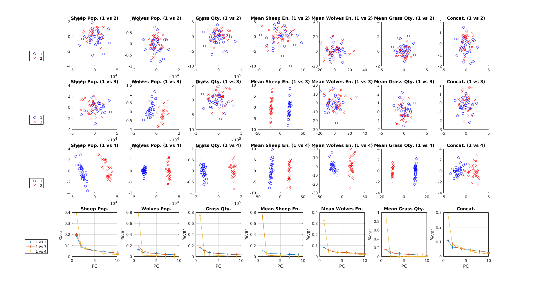
The first three rows contain the PCA score plots for the first two principal components. The last row shows the variance explained by the first ten PCs for each comparison. Irrespective of row, plots in a column are associated with the same output. Again, it is possible to observe that the compared implementations are increasingly dissimilar when going from comparison 1 to comparison 3.
Finally, setting the first parameter to 0 will return the source code for a LaTeX table. It is also convenient to redefine the output labels to better LaTeX styling:
outputs = {'$P^s$', '$P^w$', '$P^c$', '$\overline{E}^s$', ...
    '$\overline{E}^w$', '$\overline{C}$', '$\tilde{A}$'};
micomp_show(0, c, outputs, comparisons)
After compiling the returned code in a LaTeX document, the table will show as follows:

Note that LaTeX tables generated with micomp_show require that the fontenc
(with T1 option), multirow, booktabs, ulem (with normalem option) and
tikz (with plotmarks library) packages be included in the LaTeX document.
For quick testing LaTeX table generation, a template
document is provided in the templates
folder. Simply replace the commented block with the generated LaTeX code for
the table and compile the document.
micompm has the following limitations when compared with the original R implementation [2]:
- It does not support outputs with different lengths.
- It does not directly provide p-values adjusted with the weighted Bonferroni procedure.
- It is unable to directly apply and compare multiple MANOVA tests to each output/comparison combination for multiple user-specified variances to explain, although this can be achieved via multiple calls to micomp.
- The generated LaTeX tables have limited configurability via micomp_show function arguments.
The micompm unit tests require the MOxUnit framework. Set the appropriate
path to this framework as specified in the respective instructions, cd into
the tests folder and execute the following instruction:
moxunit_runtests
The tests can take a few minutes to run.
- [1] Fachada N, Rosa AC. (2018) micompm: A MATLAB/Octave toolbox for multivariate independent comparison of observations. Journal of Open Source Software. 3(23):430. https://doi.org/10.21105/joss.00430
- [2] Fachada N, Rodrigues J, Lopes VV, Martins RC, Rosa AC. (2016) micompr: An R Package for Multivariate Independent Comparison of Observations. The R Journal 8(2):405–420. https://journal.r-project.org/archive/2016-2/fachada-rodrigues-lopes-etal.pdf
- [3] Fachada N, Lopes VV, Martins RC, Rosa AC. (2017) Model-independent comparison of simulation output. Simulation Modelling Practice and Theory. 72:131–149. http://dx.doi.org/10.1016/j.simpat.2016.12.013 (arXiv preprint)
- [4] Fachada N, Lopes VV, Martins RC, Rosa AC. (2015) Towards a standard model for research in agent-based modeling and simulation. PeerJ Computer Science 1:e36. https://doi.org/10.7717/peerj-cs.36