This Get Started guide is intended as a quick way to start programming with geemap and the Earth Engine Python API.
Geemap has six plotting backends, including folium, ipyleaflet, plotly, pydeck, kepler.gl, and heremap. An interactive map created using one of the plotting backends can be displayed in a Jupyter environment, such as Google Colab, Jupyter Notebook, and JupyterLab. By default, import geemap will use the ipyleaflet plotting backend.
The six plotting backends do not offer equal functionality. The ipyleaflet plotting backend provides the richest interactive functionality, including the custom toolset for loading, analyzing, and visualizing geospatial data interactively without coding. For example, users can add vector data (e.g., GeoJSON, Shapefile, KML, GeoDataFrame) and raster data (e.g., GeoTIFF, Cloud Optimized GeoTIFF [COG]) to the map with a few clicks (see Figure 1). Users can also perform geospatial analysis using the WhiteboxTools GUI with 468 geoprocessing tools directly within the map interface (see Figure 2). Other interactive functionality (e.g., split-panel map, linked map, time slider, time-series inspector) can also be useful for visualizing geospatial data. The ipyleaflet package is built upon ipywidgets and allows bidirectional communication between the front-end and the backend enabling the use of the map to capture user input (source). In contrast, folium has relatively limited interactive functionality. It is meant for displaying static data only. Note that the aforementioned custom toolset and interactive functionality are not available for other plotting backends. Compared with ipyleaflet and folium, the pydeck, kepler.gl, and heremap plotting backend provides some unique 3D mapping functionality. An API key from the Here Developer Portal is required to use heremap.
To choose a specific plotting backend, use one of the following:
import geemap.geemap as geemapimport geemap.foliumap as geemapimport geemap.deck as geemapimport geemap.kepler as geemapimport geemap.plotlymap as geemapimport geemap.heremap as geemap
conda activate gee
jupyter notebookimport ee
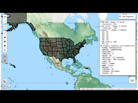
import geemapMap = geemap.Map(center=(40, -100), zoom=4)
Mapdem = ee.Image('USGS/SRTMGL1_003')
landcover = ee.Image("ESA/GLOBCOVER_L4_200901_200912_V2_3").select('landcover')
landsat7 = ee.Image('LANDSAT/LE7_TOA_5YEAR/1999_2003')
states = ee.FeatureCollection("TIGER/2018/States")dem_vis = {
'min': 0,
'max': 4000,
'palette': ['006633', 'E5FFCC', '662A00', 'D8D8D8', 'F5F5F5']}
landsat_vis = {
'min': 20,
'max': 200,
'bands': ['B4', 'B3', 'B2']
}Map.addLayer(dem, dem_vis, 'SRTM DEM', True, 0.5)
Map.addLayer(landcover, {}, 'Land cover')
Map.addLayer(landsat7, landsat_vis, 'Landsat 7')
Map.addLayer(states, {}, "US States")Once data are added to the map, you can interact with data using various tools, such as the drawing tools, inspector tool, plotting tool. Check the video below on how to use the Inspector tool to query Earth Engine interactively.