The roles of confidence in machine learning

I - What is confidence

I'm partial towards the skeptic philosophical tradition, which means I ascribe to the idea that one can't be truly confident about anything, among those is the definition of "confidence".

I've researched the commonly accepted layman definition for confidence (the first line of text that pops up when I google "confidence"):

The feeling or belief that one can have faith in or rely on someone or something

You know that a concept is fuzzy when "feeling" is used to describe it. But this one has "feeling", "faith" and "belief" in a single sentence. The only words missing to get into the top 5 most unrigorous sentences are "quantum", "consciousness", and "intuition".

What about a more formal definition?

In an ideal world where I can measure the outcome of infinite binary events I can say:

• Confidence is the probability of an event coming true, such that given an infinite number of potential events, each with a confidence from 0 to 1 assigned to them, the mean of the confidences will be equal to the fraction of events that came true.

But I'm pretty sure that this ideal world contains an ideal analytic philosopher with a panache for set-theory that would have some complaint about my use of infinity.

I'm fairly sure there is a horrible middle ground between these two definitions that relies on the well-known fact that everything in the world is a variation of the normal distribution and is thus able to give a definition that is more mathematically complex and equally impractical.

At any rate, we don't live in an ideal world and I don't need an ideal confidence. I just need a number that goes from 0 to 1, describing the approximate probability of something being true, such that if the number is 0.9999...9 I can gamble my life on the thing being true.

More pragmatically, confidence should be a value that allows me to pick a subset of predictions with average confidence x and be fairly certain that the average accuracy of those predictions will be around x.

However, I think the exact definition I want for my confidence depends on the problem I'm solving.

Speaking of which...

II - The role of confidence in Machine Learning

Does confidence have any role to play in machine learning?

Are confidence determination models useful? If so, how and why?

Is confidence a useful tool in our ontology at all or should we eat it up inside some other more useful concept?

I think confidence as defined above can be thought of as playing several roles.

1. A value by which we weight our predictions

Suppose we have a uniform target with 3 values: A, B, C. In the case of B and C the "cost" of a false positive is equal to the cost of a true positive, however, the "cost" of classifying something as A incorrectly is so great that it's equal to the benefit of 3 correct classifications of A. There are two ways to go about solving this issue:

• Negatively weighting A during training. For example, using a criterion with 3+epsilon greater penalty for miss-classifying something as A than for classifying A as something else.
• Obtaining a confidence value for our prediction, only trust predictions of A with a confidence above 75%.

Once we have a confidence (c), we can rephrase each prediction of A as: A = Pred_A | c > c_lim , null | c <= c_lim, where c_lim=3/4. Thus for every A we predict we can be assured that the cost function we are maximizing for is > 1.

Even if the confidence doesn't translate into real-world probabilities (due to training data scarcity, imperfect models and overfitting), we can still obtain a sample (C) of all confidences on the validation dataset and define c_lim such that P(True|Pred_A) > 3/4 | (A | C > c_lim ).

Even if our validation dataset is too small to trust this approach we can defensively set c_lim higher than the value determined on the validation set.

The confidence-based approach seems superior since:

• It doesn't bias the model based on some external cost function that might later change. Given a change in the TP/FP cost balance for A, we can reflect this in our predictions by just tweaking c_lim.
• It allows to quick tweaking if production data doesn't match behavior on validation data. Given that our decided upon c_lim yield accuracy < 0.75 on the production data we can try and increase c_lim until we get the desired accuracy (without retraining the whole model).
• It allows us to predict unknowns. If we bias the loss function we are still misclassifying A as B or C to avoid the large cost of a FP for A. In the confidence case, if our confidence is too small we can instead just say "I think this is likely an A but I'm not confident enough for it to be worth treating as such".

2. A value that can increase accuracy on a task where we can refuse to make some predictions

A quick and dirty example here is obviously the stock market. We have a model that predicts Y as the change in a stock's price in the next 15 minutes, for any given stock every 15 minutes. We might be making ~8000 predictions with our model, but we only need 2-3 correct predictions coupled with no false predictions to achieve our goal (get silly rich). In this hypothetical we can take only e.g. Y | c > 0.8. Thus turning even a bad model into a potentially great model assuming that said model is capable of making a few good predictions and our confidence determination is on point.

*Conversely, not many people can do this, so based on this particular example I think it's fair to speculate something like: "The kind of data that yield very imperfect models are likely to also yield very imperfect confidence determination algorithms and/or have no edge cases where the confidence can be rightfully determined as very high". *

But this is a speculation, not a mathematical or otherwise rigorous stipulation, not even a good syllogism.

To formalize this a bit more, we can define the following "cost function" for deploying our algorithm into production:

cost = prediction_error*inverse_log_func(pct_predictions_made)

By inverse_log_func I mean any scaling factor that will reduce cost if more predictions are made at less than linear rate. To get back to the stock model, assume that we are predicting in 3 situations:

1. We predict the price change for all stocks and have a prediction_error=0.5
2. We predict the price change for 0.4 of all stocks and have a prediction_error=0.2
3. We predict the price change for 0.1 of all stocks and have a prediction_error=0.05

Let's compute the cost using inverse_log_func=1/ln(1+100n):

1. cost(1) ~= 0.11
2. cost(2) ~= 0.05
3. cost(3) ~= 0.02

In a case like this a confidence determination mechanism and increase the overall performance of a model without needing to improve the model itself, potentially even in a case where we can find "no way" of improving the model.

This is more or less a generalization of case 1, but I think it's useful to keep both of them in mind.

Looking at this generic example confidence seems fairly promising, it allows us to say:

A confidence determination that's better than the overall accuracy score can improve a model past the point where it's overall usefulness scales better with increased accuracy than with the number of predictions it can makes

3. A value or mechanism for training and choosing a model

Supposed we have several models that can make predictions as an ensemble and on their one they have about equal accuracy or suppose that we want to pick between several models that all obtain around the same accuracy when cross-validated on the relevant data.

In the first case, we basically have to weight each model in the ensemble by 1/n, in the second case, we have to pick a model at random.

But suppose that we instead have a separate confidence model trained alongside each model.

In the ensemble case, training this confidence model alongside our normal models can yield a confidence that a given model in the ensemble is making a correct prediction. Assume a situation with n labels and n model for which Mx is 0.9 good at predicting x when it appears and and 1/n accurate at predicting any other label, all other models are 1/n good at predicting all other labels.

Normally, this model would be close to random, however, provided that our confidence is 100% correct our formula for picking a prediction for when Mx predicts x becomes:

[0 0 ... 1 ... 0] * 0.9 + 1/n * other_pred_vectors
[1 2 ... x ... n]

Which basically means that for 1 < n < 11 we are guaranteed to get 90% accuracy for predicting x and the accuracy stays better than random for bigger ns (though surprisingly enough the computations for this case aren't very easy)

Obviously, this is a made-up case, assuming ensemble models predict randomly defeats the point of an ensemble, but going from P(correct|X)=1/n to P(correct|X)=0.9 is a fairly huge leap by just adding a confidence value. I'm fairly sure this still holds if P((correct|x)|Pred(Mx)=x)=0.9 for any Mx for x in (1..n), but the proof is a bit harder here. However, in this case, the behavior would be closer to what we would expect from a "real" ensemble model.

The second case is a bit trickier, but we can assume a sort of "overfitting" when we pick the model out of a multitude. Assume we have a training methodology that draws out a "best candidate" on some validation set that we are constantly evaluating models on during training. Do this enough time and you end up overfitting the validation set.

However, assume that instead of evaluating the accuracy on the validation set we also evaluate the confidence. Given that confidence and accuracy are independently determined, the chance of both overfitting a validation set at the same time is 1/n where n is the number of checks we run against our validation set.

Thus, if instead of our model picking methodology being "best model on the validation set" it becomes "best model with top 80th percentile accuracy and 80th percentile confidence on the validation set". At least on an intuitive level, this seems like it could prevent overfitting on the validation data.

---

I should note the roles of confidence are not confidence-specific.

From the above I can summarize that a confidence value can help us:

1. Select a subset of predictions with higher accuracies under various scenarios
2. Modify the behavior of our predictive models both during training and during inference

But a lot of things to do (2) and (1) seems like something that could be inherent in our very models and thus needn't require a complex confidence determination mechanism. Some examples of (1) are: determining categorical certainty by looking at the non-max values in the one-hot output vector, using a quantile loss to determine a confidence range instead of an exact value for numerical predictions, predicting linear instead of binary values in order to determine likelihoods for the outcome predicted.

III A detour into confidence and explainability

I'd argue that a confidence determination mechanism can be interesting based on the inputs we feed into it, 3 different things can determine confidence.

First, let's define a few terms, we have inputs (X), outputs (Y), which for the sake of argument we can just treat as a label for each input sample. We have a machine learning model (M) trying to infer a relationship between the two, the predictions of which we will denote Yh

As such, after a prediction is made, confidence can be determined based on the values of 3 entities X,Yh, and M.

Let me give some intuitive examples of how these 3 things can be used to infer confidence:

For example, we can take X and say something like: "Oh, the SNR here looks horrible based on <simple heuristic that's hard to built into M>, let's assign this a low confidence".

We can also look at Y and say something like: "Oh, M is usually accurate, but currently Yh is an that only appears 2 times in the training data and that M was wrong every time it predicted, so let's assign a low confidence".

We can also look at M itself and say something like: "Oh, the model's activations usually match these clusters of patterns, but the current activations look like outliers, this behavior is very different from what we've previously seen so let's assign a low confidence".

Granted, both Y and M stem from X, but independently analyzing them might lead to results that are easier to act upon:

"This one pixel on the dog image looks kinda weird" is less useful to say than "The n-th layer of your model has unusually high activations due to this random pixel". Both statements are hard to act upon, but at least there's some chance of being able to make meaningful change based on the second (e.g. use some kind of regularization to normalize whatever is happening in the n-th layer).

This is all fine and dandy except that, well, there's no way to know which of the two things are "easier to act upon" in a given scenario, outside of contrived examples.

Thus, even though confidence might play a role in explainability, but the confidence determination mechanism would have to be designed with an explainability component in order for this to happen. It's not obvious that this is easier than just designing M itself with explainability capabilities built-in. However (see above), I'd tend to think that in most cases, if a confidence model can converge well on a problem, so can a predictive model, thus the confidence/explainability components lose a lot of their usefulness.

IV Confidence and training

A more interesting role of confidence determining models would be for then to serve as secondary cost generators for our models.

Does this seem silly, unintuitive, or counter-productive? Well, consider this:

Take M and a confidence determining model C that takes Yh and produces a confidence Yc. We'll train M by using some function that incorporates both M's loss function and the costs propagated from the input layer of C (in which we input Yh).

C is trained to generate a confidence value, let's just say C is trying to a number from 0 to 1 equal to the numerical value of Yh == Y (0 for false and 1 for true).

Sounds a bit strange, but let me propose a different scenario:

What if C were to just be discriminating between its inputs being Yh and it's inputs being Y, i.e. trying to discriminate between true labels and labels inferred by M.

Then, we could backpropagate the cost of this binary decision through C and into the output layer of M.

What I'm describing is basically just the training methodology for a GAN. Those seem to work stellarly well.

In addition to that, unlike GANs, we have the option of feeding the activation of any of the intermediary layers of M, as well as X, into C. Granted, I can't find experimental evidence that this should work, but at least intuitively it seems like it could be an extra useful datapoint.

The advantage this has over GANs is that C is not working against M, it's just trying to predict it's behavior. Minimizing the loss for C (having it be better able to predict if Yh == Y) will not necessarily negatively affect M's performance.

With GANs there is a risk of G being sufficiently good, but just facing off against a very well trained D that pays close attention to minute features that can't be perfectly replicated by G given such a large SNR in the loss function. However, with this approach, there's little incentive for C to behave in ways that increase the loss of M.

On the whole, this is rather promising contextual evidence and good directions to start digging further into this topic with some experimenting.

Experiments with confidence determining networks

I Experimental setup

All the code and data can be found here: https://github.com/George3d6/Confidence-Determination

If you want to but are unable to replicate some of this let me know. Everything random should be statically seeded so unless something went wrong you'd get the exact same numbers I did.

---

In order to ruminate on the idea of confidence determination I will do the following experiment:

Take a fully connected network (M) and train it on 4 datasets:

The first dataset (a) is a fully deterministic dataset dictated by some n-th degree polynomial function:

f(X) = c1 \* X[1]^1 + ... cn * X[n]^n

Just to keep it simple let's say ck = k or ck = (n+1-k)

We might also play with variation of this function where we remove the power or the coefficient (e.g. f(X) = 1*X[1]...n*X[n] and f(X) = X[1]^1 + ... X[n]^n). The choice is not that important, what we care about is getting a model that converges almost perfectly in a somewhat short amount of time.

We might also go with an even simpler "classification" version, where f(X) = x % 3 if x < 10 else None for x in X, thus getting an input of only 0, 1 and 2. Whichever of these 3 labels is more common, that's the value of Y.

The value to be predicted, Y = 0 | f(x) < lim1, 1 | lim1 < f(x) < lim2, 2 | lim2 < f(x)

lim1 and lim2 will be picked such that, for randomly generate values in X between 1 and 9, the split between the potential values of Y in the dataset is 33/33/33.

---

The second dataset (b) is similar to (a) except for the value of Y, which is:

Y = 0 | f(x) < lim1, 1 | lim1 < f(x)

But, given some irregularity in the inputs, say X[0] == 5 => Y = 2

lim1 will be picked such that the initial split is 50/50, given that we are using the 1st degree variable to introduce this irregularity in 1/9th of samples, I assume the final split will be around 11/44.5/44.5.

---

The third dataset (c) is similar to (a) except that the when Y == 2 there's a 1/3 chance that Y will randomly become 0.

---

These 3 dataset are symbolic, though obviously not fully representative of 3 "cases" in which I'd like to think about the idea of confidence:

a) Represents a case where the datasets follows a straight forward equation which, in theory, the model should be able to approximate with ~100% accuracy.

b) Represents a case where the datasets follows a deterministic equation, but this equation has an irregularity which breaks it's linearity in several places, which seem "random" when looking at the final value but obvious when looking at the input independently.

c) Represents a case where noise is added to the data, such that 100% accuracy can't be reached. However, assuming a perfect model, we know the confidence we should have in our predictions: P(correct|1) = 1, P(correct|0) = 75, P(correct|2) = 66.

I want to test some solutions here and evaluate them based on six criteria:

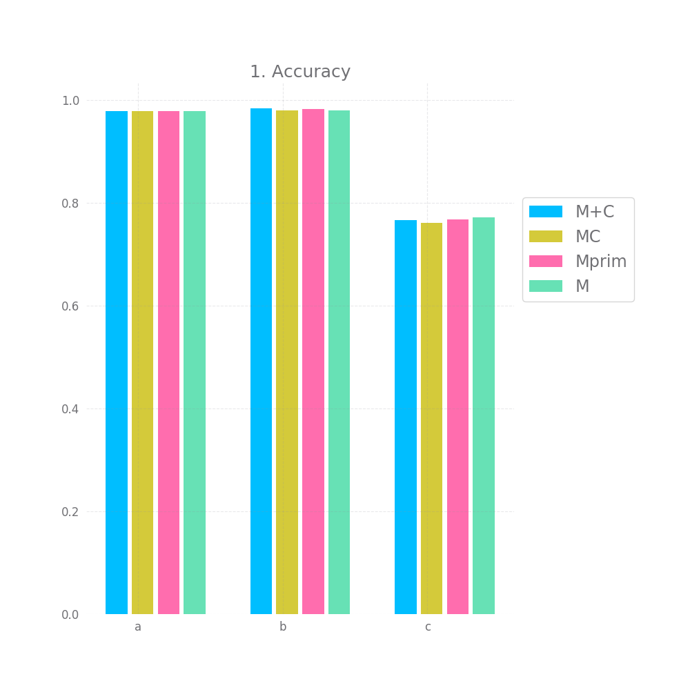
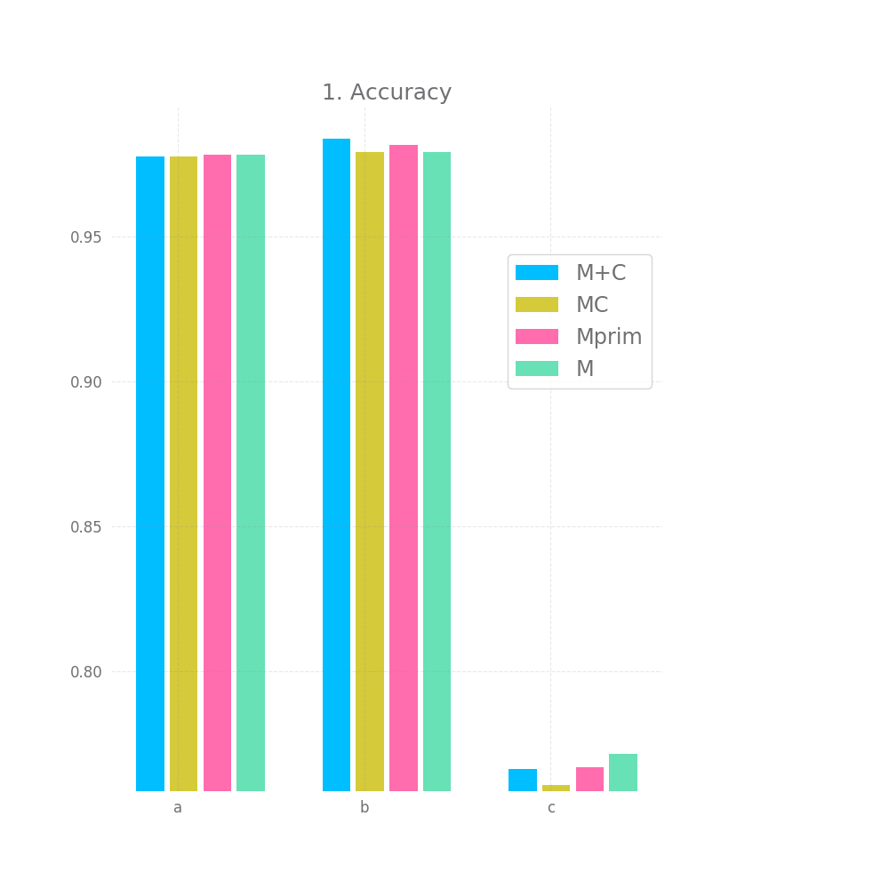
1. Accuracy, overall accuracy achieved on a testing datasets generated by the same process as the original ones.
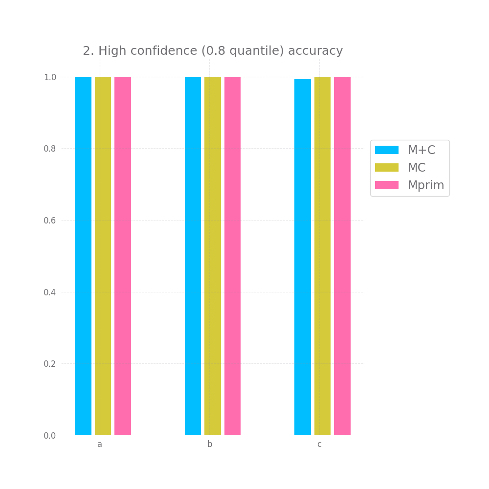
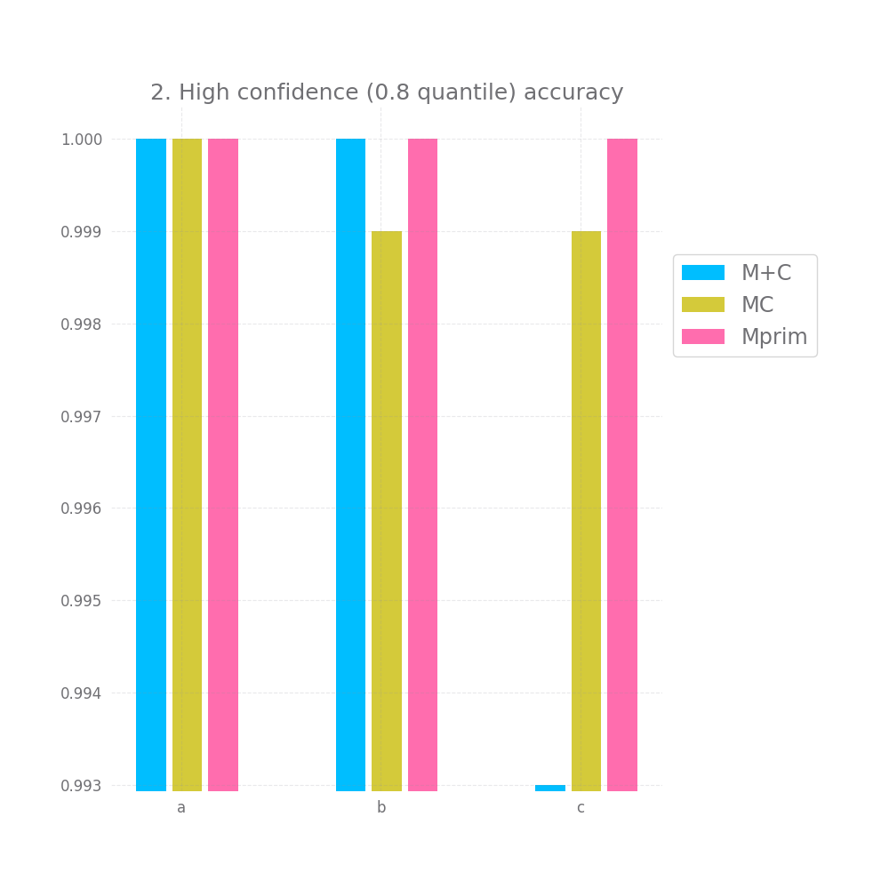
2. Given that I only pick predictions with high confidences (say 0.8 quantile), how high is the accuracy for this subset of predictions ?
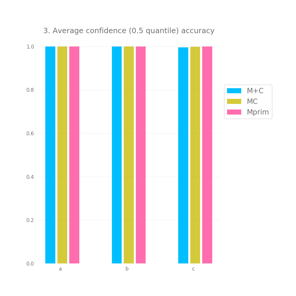
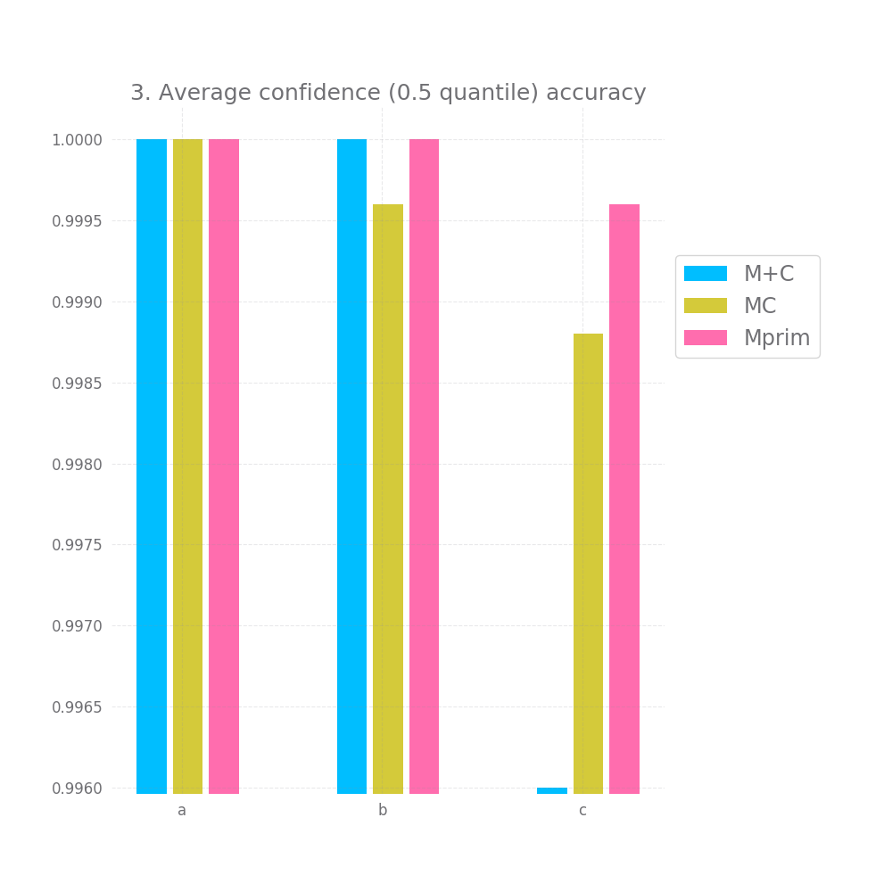
3. Given that I only pick predictions with above average confidences (say 0.5 quantile), how high is the accuracy for this subset of predictions ?
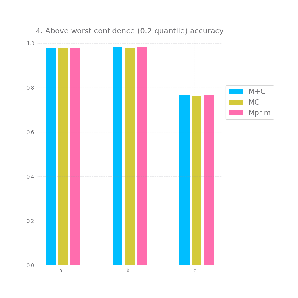
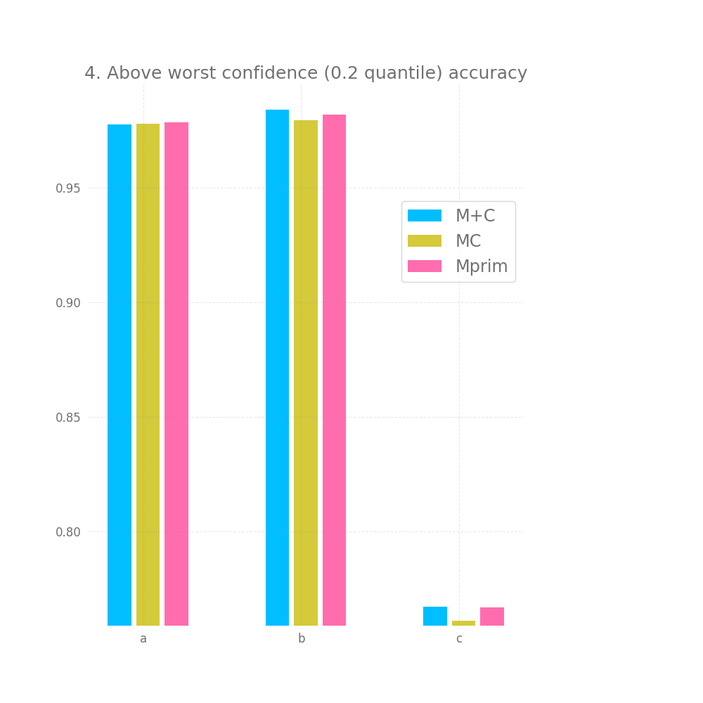
4. Given that I only all pick predictions but those with the lowest confidences (say 0.2 quantile), how high is the accuracy for this subset of predictions ?
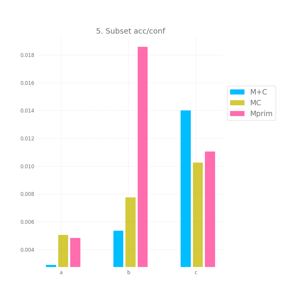
5. Given a random subset of predictions + confidences, is the mean of the confidence values equal to the accuracy for that subset of predictions ?
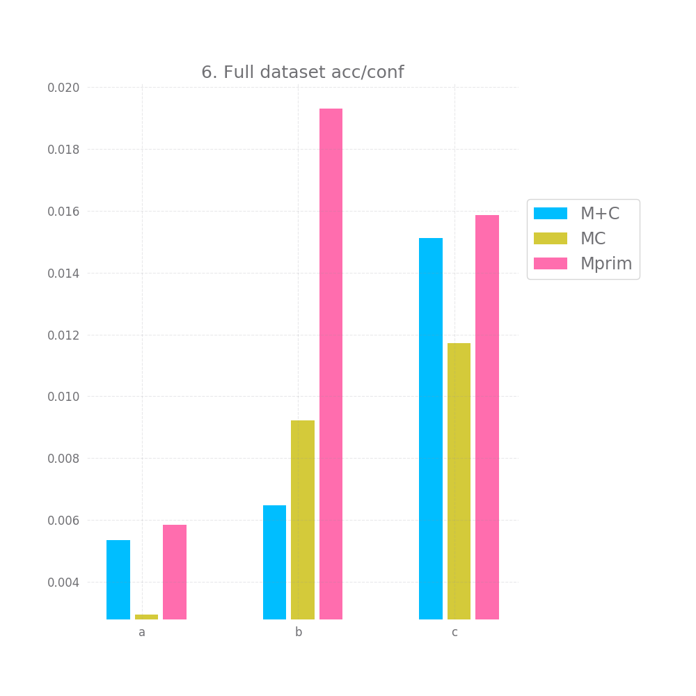
6. same as (4) but on the whole dataset rather than a random subset.
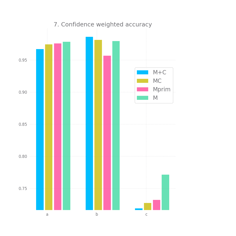
7. Assuming a situation where a wrong predictions is -1 and a correct prediction 1, and the accuracy score is the sum of all these -1 and 1 values. Would weighting this value by their associated confidence increase the value of this sum ?
8. How long does the setup take to converge on a validation dataset ? For ease of experimenting this means "how long does the main predictive model take to converge", once that converges we'll stop regardless of how good the confidence model has gotten. This will also be capped to avoid wasting too much time if a given model fails to converge in a reasonable amount of time compared to the others.
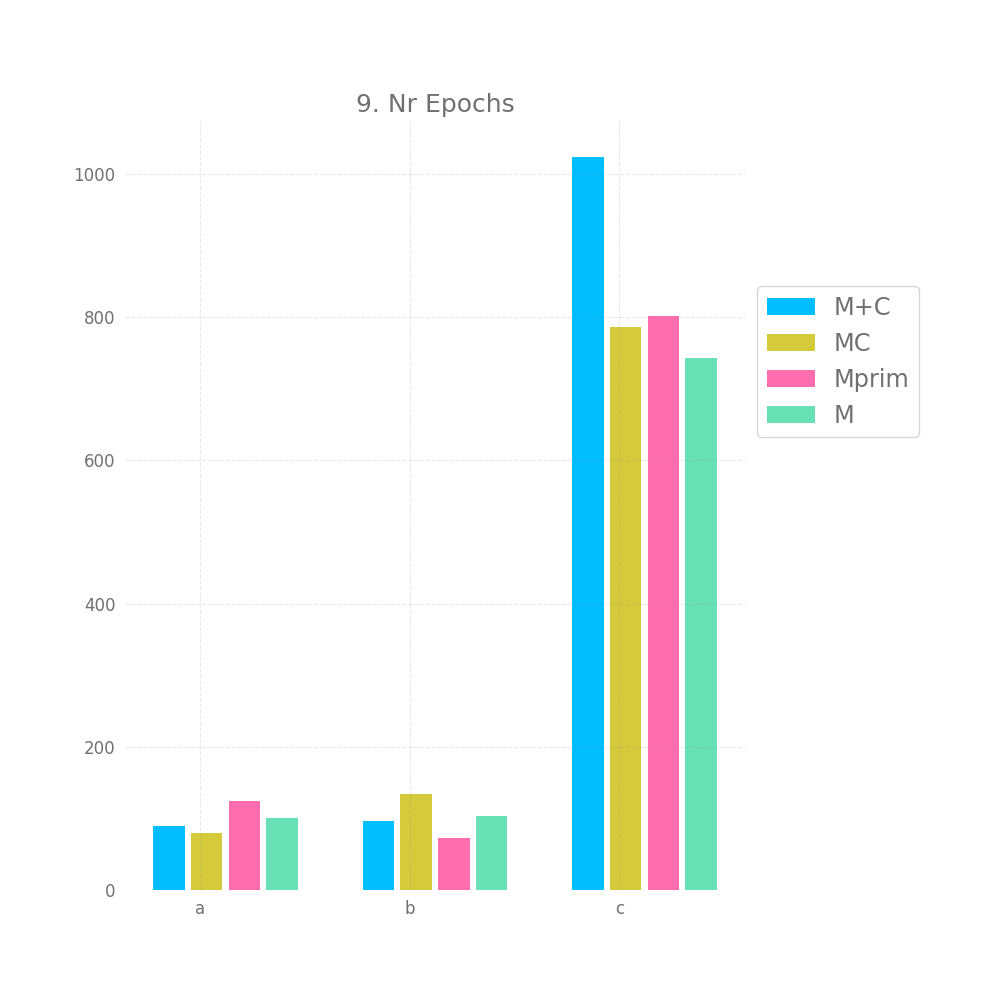
9. The number of epochs it takes each model to converge.

The models evaluated will be:

• Just letting M predict, no confidence involved.

• Let M predict and have a separate model C that predicts the confidence (on a scale from 0 to 1) based on the inputs X and Yh.

• Let a different model M' predict, this is a model similar to M but it includes an additional cell into the outputs for predicting a confidence value and some additional cells evenly distributed in all layers in order to have an M' training in roughly equal time to that of M + C.

• Let M predict and have a separate model C that predicts the confidence just like before, however, the loss from the Yh component of the last layer of C is backproped through M.

---

I will run each model through all dataset and compare the results. Running model M alone serves as a sanity benchmark for the accuracy values and is there in order to set the maximum training time (4x how long it take to "converge" on validation data) in order to avoid wasting too much time on setups that are very slow to converge (these would probably be impractical).

I will also use multiple datasets, the combinations will be:

1. Degree: 3 ,4 ,5 ,and 6
2. Function: linear, polynomial ,and polynomial with coefficients

For each dataset I will generate a training, validationa and testing set of equal size, consisting of either ~1/3 of all possible combinations or 10,000 observations (whichever is smaller), without any duplicate values in X.

Barring issues with training time I will use the 6th degree polynomial with coefficients as my example, as it should be the most complex dataset of the bunch.

Though, I might use the other examples to point out interesting behavior. This is not set in stone, but I think it's good to lay this out beforehand as to not be tempted to hack my experiment in order to generate nicer looking results, I already have way too many measures to cherry pick an effect out of anyway.

II The results

A few days later, I have some results:

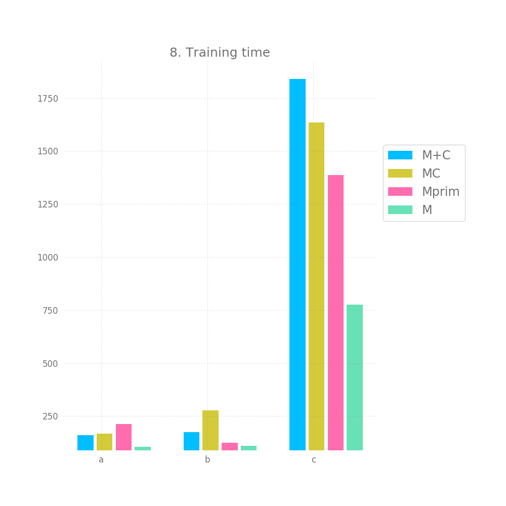
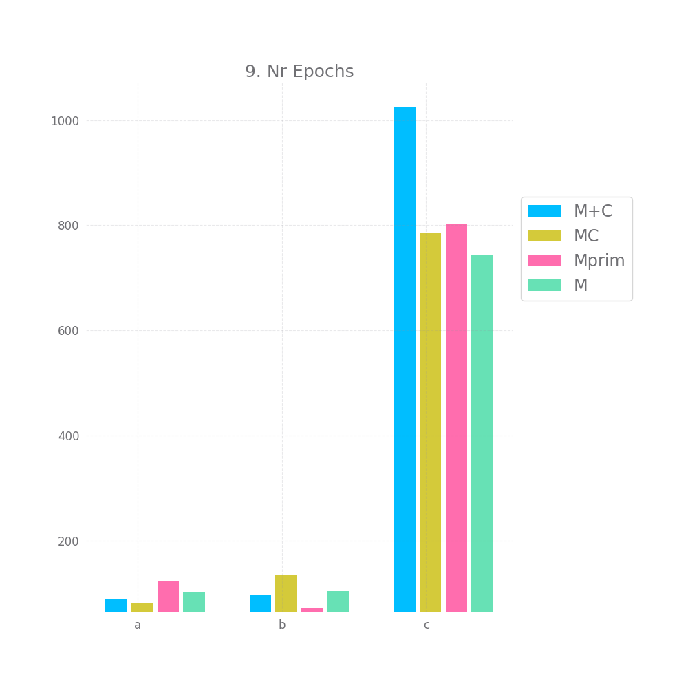
Here they are (for the 6th degree polynomial with coefficients dataset):

Let's explore these one by one:

In terms of raw accuracy, all models performed basically the same, there's some difference, but considering there's some difference between M+C and M, sometimes with M's accuracy being lower, I think it's safe to think of these small differences as just noise.

This is somewhat disappointing, but to be fair, the models are doing close-to-perfect here anyway, so it could be hard for Mprim or MC to improve anything. Well, except for the c dataset, in theory one should be able to get an accuracy of ~89% of the c dataset, M's accuracy however is only 75%. So one would expect this is where Mprim or MC could shine, but they don't. There's a 1% improvement with Mprim and even an insignificant drop with MC compared to M.

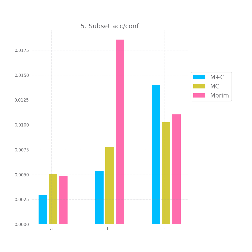
There's a bit of hope when we look at graph nr 2 and 3 measuring the accuracy for high and medium confidence predictions. On all 3 datasets and for all 3 approaches both of these are basically 100%. However, this doesn't hold for graph nr 4, where we take all but the bottom 20% predictions in terms of confidence, here we have a very small accuracy improvement, but it's so tiny it might as well be noise.

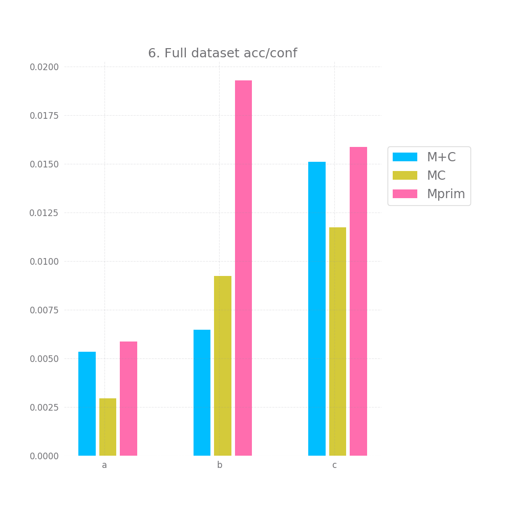
Graph 5 and 6 look at how "correct" the confidence is on average. Ideally the mean confidence should be equal to the accuracy. In that case, both these graphs would be equal to 0.

This is not quite the case here, but it's close enough, we have difference between 0.2 and 1.4% between the mean confidence and the accuracy... not bad. Also, keep in mind that we test this both on the full testing datasets and a random subset, so this is likely to generalize to any large enough subset of data similar to the training data. Of course, "large enough" and "similar" are basically handwavey terms here.

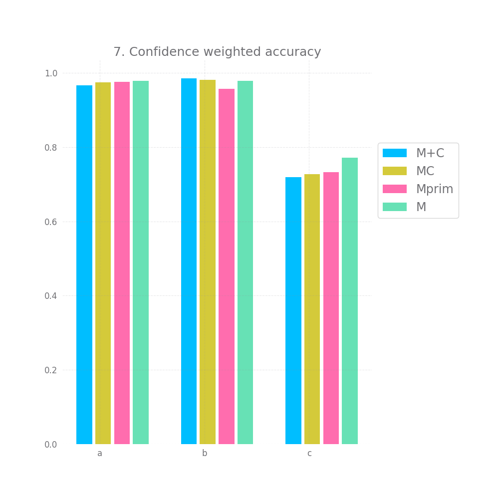
Lastly, we look at 7 and observe that weighting the accuracy by the confidence doesn't improve accuracy, if anything it seems to make it insignificantly smaller. There might be other ways to observe an effect size here, namely only selecting values with a low confidence, but I'm still rather disappointed by this turnout.

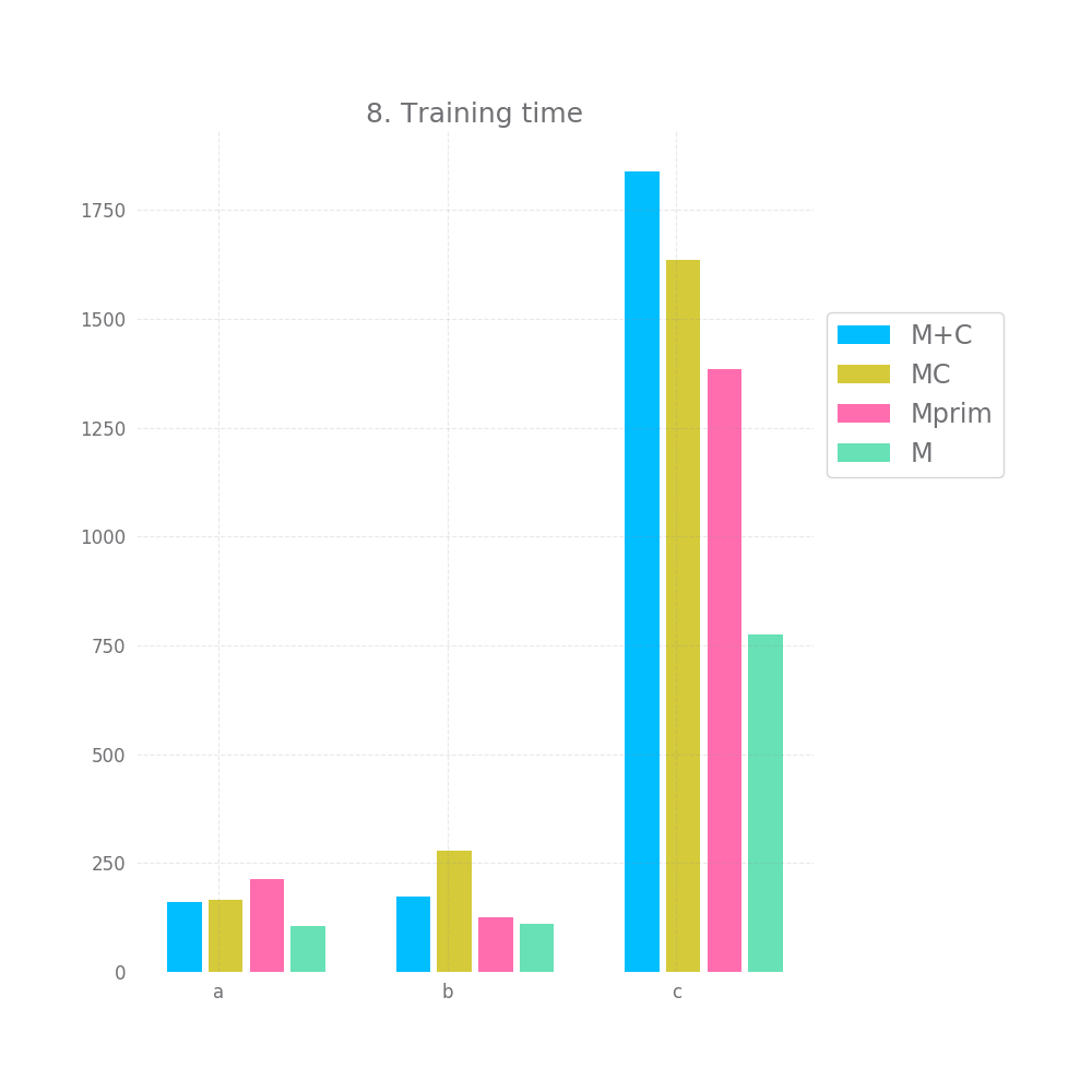
Finally, the training time and number of epochs is unexpected, I'd have assumed Mprim takes the longest to converge, followed by MC and that M+C is the fastest. However, on the c dataset we observe the exact opposite. This might serve as some indication that MC and Mprim are able to "kind of figure out" the random element earlier, but I don't want to read too much into it.

Let's also take a look at the relative plots:

III A broader look at the results

Ok, before I draw any conclusion I also want to do a brief analysis of all the datapoints I collected. Maybe there's some more signal in all that noise.

Again, remember I have datasets a,b and c generated using a linear polynomial and polynomial-with-coefficients formula for degrees 3,4,5 and 6. That's 44 more datasets to draw some conclusions from.

I'm going to average out all the scores per model for each dataset and for all dataset combined to see if I find any outliers. I also tried finding scores that were surprisingly high (e.g. MC performing 10% better than M+C and Mprim on a specific dataset) but couldn't find any, however feel free to run the code for yourself and dig thorugh my results or generate your own.

That aside being said:

1. On all datasets combined

M+C performs better by 1-4% on all accuracy metrics metrics: Accuracy, High confidence accuracy, Average confidence accuracy, Above worst confidence accuracy. Next comes MC and Mprim is the worst of the bunch by far (MC and M+C are within 1-2%, Mprim is 3-6% away)

M+C and MC perform about equally on the acc/conf tradeoff both on the whole dataset and on the sample, being off by 2-3.7%. Mprim however is much worst and on average it's off by ~23%.

When we "weight" the accuracy using the confidence, the resulting accuracy is still slightly worst for all models compared to the original M. However, again, Mprim falls behind both M+C and MC.

2. On dataset of type a

The pattern for the accuracy metric change a bit, with MC being above or about the same as M+C and even managing to beat M in overall accuracy. But the difference is not that significant

Mprim peforms horribly, with errors > 45% in the accuracy/confidence tradeoff, both M+C and MC perform close to perfect, with M+C having errors ~3% and MC ~0.5%.

The story for weighted accuracy stays the same.

3. On dataset of type b

The pattern for accuracy has Mprim and M+C tied here, with MC being ~4% worst on the overall accuracy and the accuracy of the top 80% of predictions chosen by confidence (i.e. metric 4, above worst confidence).

The acc/conf metric is about the same for all models, nearing a perfect match with erros in the 0.x% and 0.0x%.

The story for weighted accuracy stays the same.

4. On dataset of type c

We've finally reached the good stuff.

This is the only dataset type that is impossible to perfectly predict, this is the kind of situation for which I'd expect confidence models to be relevant.

Average accuracy is abysmal for all models, ranging from 61% to 68%.

When looking at the accuracy of predictions picked by high confidence, for the 0.8 and 0.5 confidence quantile M+C has much better accuracy than Mprim and M+C

For above worst confidence accuracy (0.2 quantile) all models perform equall badly, at ~73%, but this is still a 5% improvement over the original accuracy.

In terms of the acc/conf metric, M+C only has an error of ~2 and ~3%, while MC has errors ~11% and Mprim has errors of ~22% and ~24%.

Finally, when looking at the confidence weighted accuracy, all 3 confidence model beat the standard accuracy metric, which is encouraging. MC does best, but only marginally better than Mprim.

However M's accuracy results on datasets of type c were really bad, when we compare the confidence weighted accuracy to the plain accuracy of e.g. MC, M+C and Mprim the confidence weighted accuracy is still slightly bellow the raw accuracy.

IV Conclusions

To recapitulate, we've tried various datasets that use a multiple-parameter equation to model a 3-way categorial label in order to test various ways of estimating prediction confidence using fully connected networks.

One the datasets was manipulated to introduce predictable noise in the input->label relationship, the other was manipulated to introduce unpredictable noise in the input->label relationship.

We tried 3 different models:

• M+C which is a normal model and a separate confidence predicting network that uses the ouputs of M and the inputs of M as it's own input.
• MC which is the same as M+C except for the fact that the cost from the Y component of the first layer of C is propagated through M.
• MPrim which is a somewhat larger model with an extra output cell representing a confidence value.

It seems that in all 3 scenarios, all 3 models can be useful for selecting predictions with higher than average accuracy and are able to predict a reliable confidence number, under the assumption that a reliable confidence, when averaged out, should be about equal to the model's accuracy.

On the above task, MC and M+C performed about equally well, with a potential edge going out to M+C. MPrim performed significantly worst on many of the datasets.

We did not obtain any significant results in terms of improving the overall accuracy using MC and MPrim, weighting the accuracy by the confidence did not improve the overall accuracy.

For MC and M+C, the average confidence matched the average accuracy with a < 0.05 error for the vast majority of datasets, which indicates some "correctness" regrading the confidence.

This is enough to motivate me to do a bit more digging, potentially using more rigorous epxeriments and more complex datasets on the idea of having a separate confidence-predicting network. Both the MC and M+C approach seem to be viable candidates here. Outputting a confidence from the same model seems to show worst performance than a separate confidence network.

V Experimental errors

• Datasets were no varied enough.
• The normal model M should have obtained accuracies of ~100% on datasets of type a and b and ~88% on datasets of type c. The acuracies were never quite that high, maybe a completely different result would have been obtained on c has M learned how to predict it as close to reality as possibe. However, this behaviour would have negated the experimental value for datasets of type a and b.
• MSELoss was used for the confidence (ups), a linear loss function might have been better here.
• The stopping logic (aka what I've referred to as "model converging") uses and impractically large validation set and it's implementation isn't very straight forward.
• The models were all trained with SDG using a small learning with. We might have obtained better and faster results with a quicker optimizer that used a scheduler.
• Ideally, we would have trained 3 or 5, instead of 1 model per dataset. However, I avoided doing this due to time constraints (the code takes ~10 hour to run on my current machine)
• For metrics like confidence weighted accuracy and especially conf/accuracy on a subset it might have been more correct to CV with multiple subsets. However, since the testing set was separate from the training set, I'm unsure this would have counted as a best practice.
• The terms of the experiments were slightly altered once I realized I wanted to measure more metrics than I had originally planned.
• There are a few anomalies caused by no value being present in the 0.8th quantile of confidence, pressumably I should have used a >= rather than > operator, but now it's too late.

On the whole, if people find this interesting I might run a more thorough experiment taking into account the above points. That being said, it doesn't seem like these "errors" should affect the data relevant for the conclusion too much, though they might be affecting the things presented in section III quite a lot.