Alaska

This repository contains replication code, data, and additional material to accompany the paper Mathematics of Nested Districts: The Case of Alaska which grew out of a project started at the 2018 Voting Rights Data Institute.

Alaska State House Districts	Alaska State Senate Districts

Pairing Districts

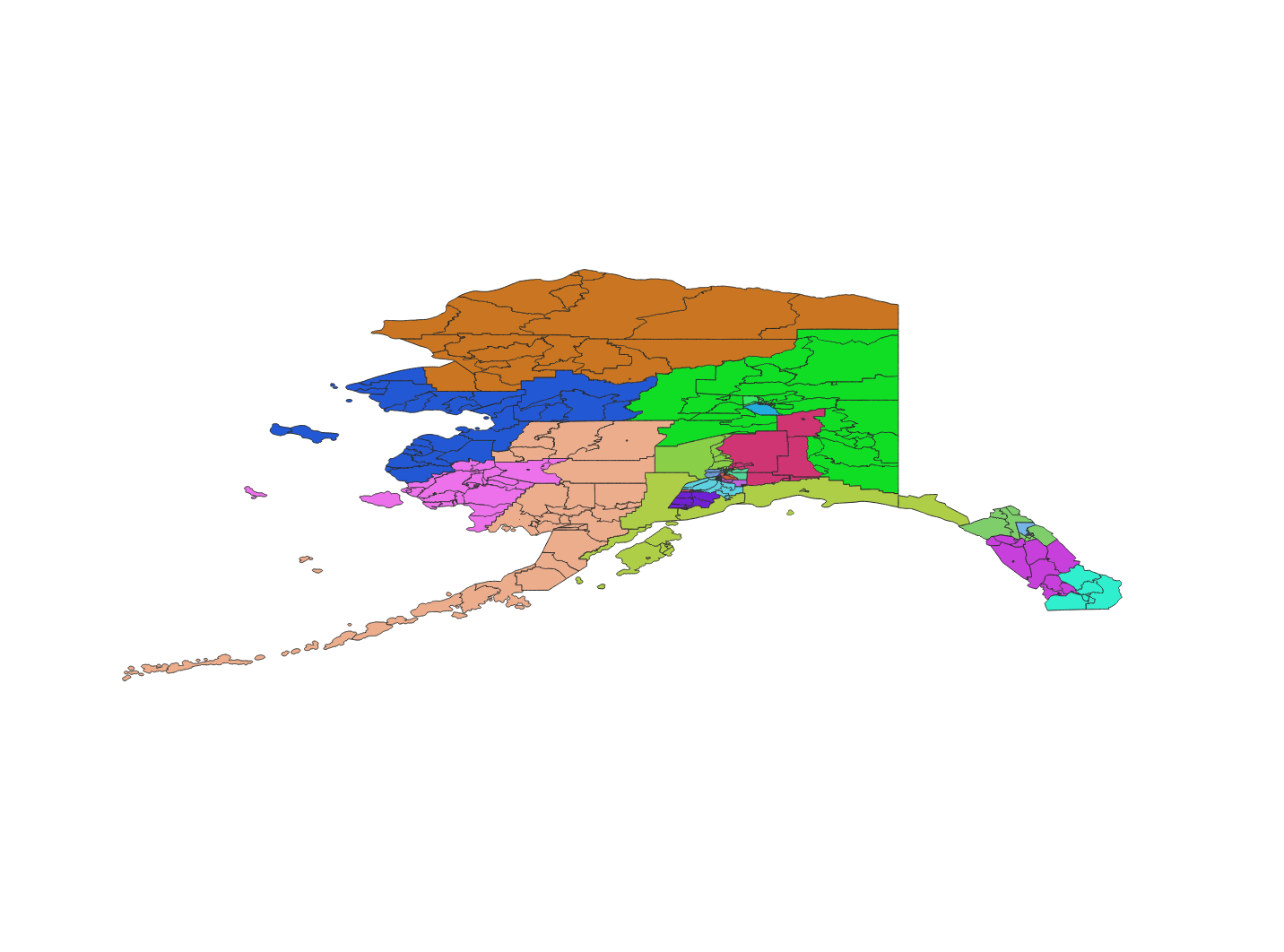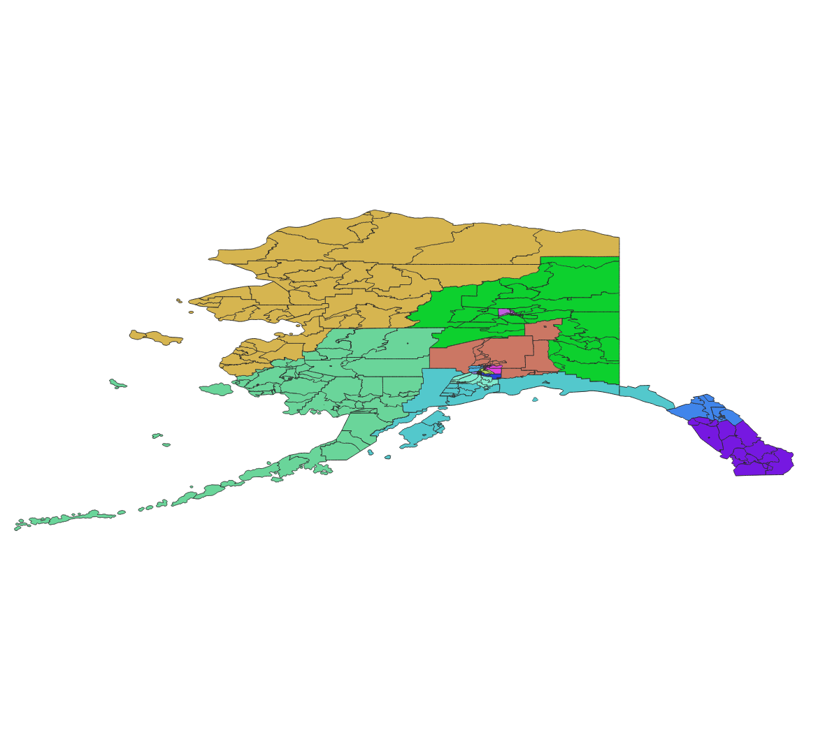This paper analyzes a pairing rule that eight states require of their state legislative districting plans - Senate districts must be formed by joining adjacent pairs of House districts. From a mathematical perspective, this is a question of constructing perfect matchings on the Dual Graph of the House districts. We focus mainly on the state of Alaska where it is possible to generate the full set of matchings and evaluate the expected partisan behavior of the associated Senate plans. To get a sense of the scale of this problem, the table below shows the number of districts and perfect matchings for each of the relevant states.

State	# House Districts	# Dual Graph Edges	# Perfect Matchings
Alaska	40	100	108,765
Illinois	118	326	9,380,573,911
Iowa	100	251	1,494,354,140,511
Minnesota	134	260	6,156,723,718,225,577,984
Montana	100	269	11,629,786,967,358
Nevada	42	111	313,698
Oregon	60	158	229,968,613
Wyoming	60	143	920,864

Alaska	Illinois	Iowa	Minnesota	Montana	Nevada	Oregon	Wyoming

Our techincal contributions include an implementation of the FKT algorithm for counting the number of perfect matchings in a planar graph, a prune-and-split algorithm for generating the matchings, and a uniform sampling implementation for analyzing states like Minnesota, where generating the full set of matchings would be prohibitively expensive. The FKT function is fast enough to incorporate at every step of the Markov chain sampling procedure for generating new House plans and forms the backbone of the uniform sampling algorithm. These techniques also allow us to investigate the relationship between the number of edges in the dual graph and the number of matchings, which is of independent mathematical interest.

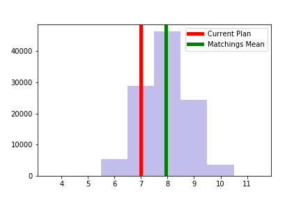
For Alaska, we show that compared to the full collection of possible matchings of the currently enacted plan the chosen pairing exhibits an approximate advantage of 1 Republican seat. Interestingly, the House districting plan appears to have a similar magnitude advantage for the Democratic party compared to a neutral ensemble formed with a Markov chain. Histograms of these results are shown below. We also verify the usefulness of our sampling techinque by comparing it to the ground truth available in Alaska and examine the extremal plans found in the Markov chain ensemble. Finally, we provide a cleaned dataset of merged geographic and partisan data and describe the choices that must be made to compile these resources.

# Democratic Senate Seats across all perfect matchings	# Democratic House Seats across 100k plans

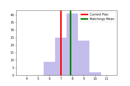
As mentioned above, we implemented a uniform sampling method for perfect matchings that allows us to analyze situations where it would be difficult to generate the entire list. In order to validate this approach we sampled 100 matchings from the 108,765 in Alaska and compare the sample distribution to the known, full distribution in the figure below. The difference between the mean of the sample distribution and the actual distributions is less than 0.1 seats. This suggests that this technique can be employed effectively, even in states with an enormous number of potential matchings.

# Democratic Senate Seats across all perfect matchings	# Democratic Senate Seats across 100 Samples

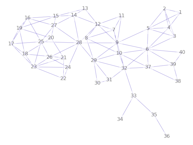
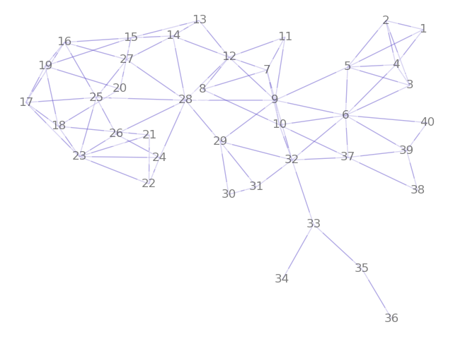
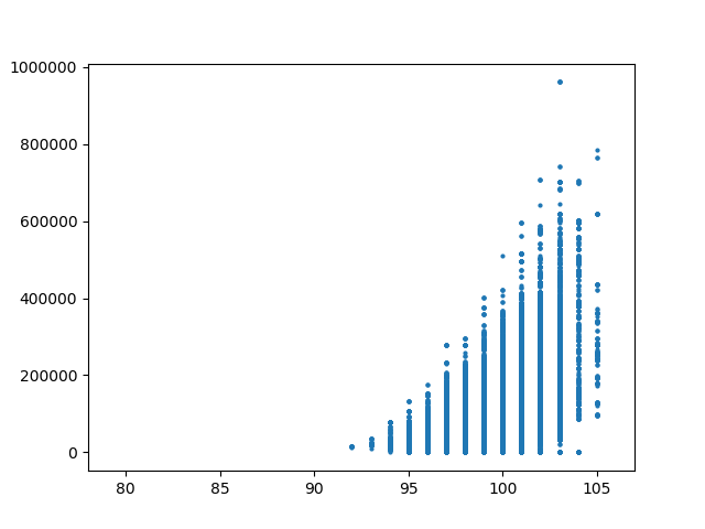
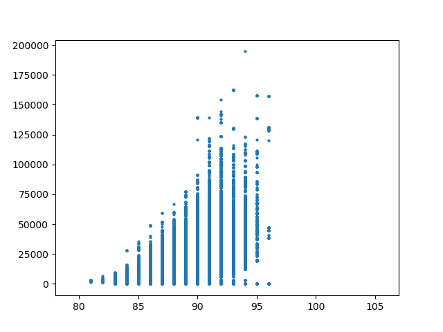
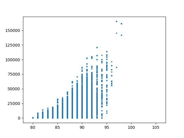
We also note some interesting structure in the relationship between the number of edges in the underlying dual graph of precicnts to the number of edges and matchings in the dual graph of House districts. The plots below show the House adjacencies for the three dual graphs considered in the paper and the plots of dual graph edges against total number of perfect matchings for each step in the ensemble, on each set of precinct adjacencies. The differences are a result of adjusting the connectivity of the precinct graph across the water around Anchorage. One of the key messages of our paper is that these seemingly small choices about water adjacency can have large impacts on the space of permissible plans.

Permissive	Restricted	Tight
100 edges	92 edges	89 edges
108,765 matchings	29,289	14,446

Replication

To reproduce the experiments in the paper begin by cloning this repository or clicking the Download ZIP option. You will also need to install Gerrychain and update NetworkX to at least version 2.3. After you have extracted the files you will need to unzip AK_precicnts_NS.zip which is in the data directory. Navigate your terminal to the main directory and enter: python matching_verification. py

The replication code does the following:

1. Begins by constructing the three dual graphs on house districts: tight, restrictive, and permissive by starting fresh from the shapefile, adding the island edges, and then deleting the water connections around Anchorage.
2. It next checks that the edges nest i.e. that tight <= restricted <= permissive.
3. Once it confirms that everything is OK, the adjacency matrices are written to Outputs.
4. Then it uses FKT to enumerate the matchings for each graph and returns the number and the running time
5. Next it generates all of the matchings for each graph and returns the running time
6. The full sets of matchings are written to file to save for later
7. Next it checks that for each of the sets of matchings, the indices correctly correspond to pairs of adjacent districts by checking that there are cut edges in the partition that correspond to each pair.
8. For each of the three graphs it loads each matching and computes the partisan balance for the elections
9. These values are also written to Outputs
10. Then it generates the box plots and histograms for seats and competitive districts, just like the ones in the paper. These are saved in Outputs/plots
11. It also writes separate text files with the averages compared to the enacted plan values, like the tables in the paper. These are saved in Outputs/values
12. It takes about 12 minutes to get to this point - having generated and analyzed all of the matchings of the enacted plan corresponding to the three graphs.
13. Next, for each of the graphs it runs 100,000 ReCom steps starting at the enacted plan.
14. At every step, it records the partisan values as well as the number of edges in the house dual graph and FKT # of matchings.
15. After it finishes each run, it generates the same box plots, histograms, and text files as the matchings version as well as the plot of edges vs. matchings.
16. Finally, the outputs are written to file and the final time is reported.

For these 100k steps runs it takes about 3 hours to do everything (shortens to 1/2 an hour if you only do 10k steps). At the conclusion of the run the plots and values folders will be populated with complete sets of outputs matching the experiments described in the paper on all three Alaska dual graphs. The program will also write timing information and validity checks to the terminal.

Subdirectories

• GerryChain contains sample code for building ensembles that we used while doing the exploratory analysis.
• Limited Adjacency contains a version of the shapefile that is clipped to the land area of the state.
• Outputs contains a zipped folder with the actual outputs analyzed in the paper as well as providing the directory structure to be populated for replication.
• Preprocessing contains code for downloading the state level shapefiles and extracting the corresponding dual graphs as .csvs.
• Summer Code contains more exploratory code an earlier versions of the main functions.
• data contains the adjacency matrices for the dual graphs and .json files for the complete matchings of the Permissive and Restricted plans. The main precinct level shapefile for Alaska is included as AK_precicnts_NS.zip.
• shapefiles contains the state level shapefiles.
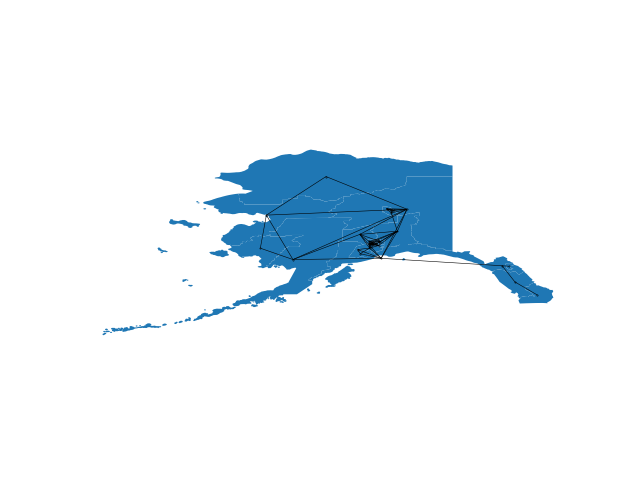
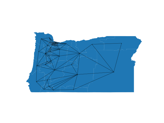
• Tests contains testing examples for the various python functions and plotting code for nearly planar embeddings like those in the paper.

Python Functions

• FKT.py provides a function named FKT that enumerates all of the perfect matchings in a given planar graph. It takes as input a numpy matrix representing the adjacencies. This can be extracted from a networkx graph object as nx.adjacency_matrix(G).todense() and the program can be called with round(FKT(nx.adjacency_matrix(G).todense()))
• enum_matchings.py provides a function names enumerate_matchings that generates a list off all of the perfect matchings of a planar graph. It takes an input a numpy array of the graph adjacencies and can be called with enumerate_matchigs(np.array(nx.adjacency_matrix(G).tolist(),list(range(len(G.nodes()))).
• uniform_matching.py provides a function uniform matching that takes as input a networkx graph object and returns a uniformly sampled perfect matching.
• The remainder of the python files perform tests and plotting features.