forked from jslefche/sem_book
-
Notifications
You must be signed in to change notification settings - Fork 0
/
05-Multigroup_models.Rmd
316 lines (194 loc) · 18.2 KB
/
05-Multigroup_models.Rmd
1
2
3
4
5
6
7
8
9
10
11
12
13
14
15
16
17
18
19
20
21
22
23
24
25
26
27
28
29
30
31
32
33
34
35
36
37
38
39
40
41
42
43
44
45
46
47
48
49
50
51
52
53
54
55
56
57
58
59
60
61
62
63
64
65
66
67
68
69
70
71
72
73
74
75
76
77
78
79
80
81
82
83
84
85
86
87
88
89
90
91
92
93
94
95
96
97
98
99
100
101
102
103
104
105
106
107
108
109
110
111
112
113
114
115
116
117
118
119
120
121
122
123
124
125
126
127
128
129
130
131
132
133
134
135
136
137
138
139
140
141
142
143
144
145
146
147
148
149
150
151
152
153
154
155
156
157
158
159
160
161
162
163
164
165
166
167
168
169
170
171
172
173
174
175
176
177
178
179
180
181
182
183
184
185
186
187
188
189
190
191
192
193
194
195
196
197
198
199
200
201
202
203
204
205
206
207
208
209
210
211
212
213
214
215
216
217
218
219
220
221
222
223
224
225
226
227
228
229
230
231
232
233
234
235
236
237
238
239
240
241
242
243
244
245
246
247
248
249
250
251
252
253
254
255
256
257
258
259
260
261
262
263
264
265
266
267
268
269
270
271
272
273
274
275
276
277
278
279
280
281
282
283
284
285
286
287
288
289
290
291
292
293
294
295
296
297
298
299
300
301
302
303
304
305
306
307
308
309
310
311
312
313
314
315
316
---
title: "Multigroup Analysis"
author: "Jon Lefcheck"
date: "November 12, 2018"
output: html_document
---
# Multigroup Analysis
## Introduction to Multigroup Analysis
Often in ecology we wish to compare the results from two or more groups. These groups could reflect experimental treatments, different sites, different sexes, or any number of types of organization. The ultimate goal of such an analysis is to ask whether the relationships among predictor and response variables vary by group. For example, does the effect of pesticide on invertebrate biomass change as function of where the pesticide is applied?
Historically, such a goal would be captured through the application of a statistical interaction. In the above example, the statistical model might be something like:
$$biomass = pesticide * location$$
Here, a significant interaction between $pesticide \times location$ would indicate that the effect of pesticide applicaiton on invertebrate biomass varies by location. It would of course then be up to the author to use their knowledge of the system to speculate why this is.
In the event that the interaction is not statistically significant, then the author would conclude that the effect of pesticide is invariant to location, and could go on to interpret the main effect of pesticide. In this situation, they are able to generalize the effects of pesticide such that it is expected to have the same magnitude of effect regardless of where it is applied.
A multigroup model is essentially the same principle, but instead of focusing on a single response, the interaction is applied across a network of variables. In other words, it asks if not just one, but *all* coefficients are the same or different across groups while leveraging the entirety of the data across groups. In a sense, it can be thought of as a "model-wide" interaction, and in fact, this is how we will treat it later using a piecewise approach.
One could simply fit the same model structure to different subsets of the data, but this would not allow you to identify *which* paths change based on the group and which do not. Rather, one would have to compare the magnitude and standard errors of each pair of coefficients manually, rather than through a formal statistical procedure.
The application of multigroup models differs between a global estimation (i.e., variance-covariance-based SEM) and local estimation (i.e., piecewise SEM), but adhere to the same idea of identifying which paths have the same effect across groups, and which paths vary depending on the group.
In this chapter, we will work through both approaches, and then compare/contrast the output.
## Multigroup Analysis using Global Estimation
Multigroup modeling using global estimation begins with the estimation of two models: one in which all parameters are allowed to differ between groups, and one in which all parameters are fixed to those obtained from analysis of the pooled data across groups. We call the first model the "free" model since all parameters are free to vary, and the second the "constrained" model since each path, regardless of its group, is constrained to a single value determined by the entire dataset.
If the two models are not significantly different, and the latter fits the data well, then one can assume there is no variation in the path coefficients by group and multigroup approach is not necessary. If they are, then the exercise shifts towards understanding which paths are the same and which are different. This is achieved by sequentially constraining the coefficients of each path and re-fitting the model.
Let's illustrate this procedure using a random example using three variables ($x$, $y$, and $z$) in two groups ("a" and "b"):
```{r}
set.seed(111)
dat <- data.frame(x = runif(100), group = rep(letters[1:2], each = 50))
dat$y <- dat$x + runif(100)
dat$z <- dat$y + runif(100)
```
In this example, we suppose a simple mediation model: $x -> y -> z$, and that all three variables are correlated to some degree so that this path model makes sense.
We can use *lavaan* to fit the "free" model. The key is allowing the coefficients to vary by specifying the `group =` argument.
```{r echo = T, results = 'hide'}
multigroup.model <- '
y ~ x
z ~ y
'
library(lavaan)
multigroup1 <- sem(multigroup.model, dat, group = "group")
```
We can then obtain the summary of the multigroup analysis:
```{r}
summary(multigroup1)
```
Note that, unlike the typical *lavaan* output, the printout is now organized by group, with separate coefficients for each path in each group. Because this model is allowed to vary, the coefficient for the $x -> y$ path in group "a" is different, for example, from that reported for group "b".
Next, we fit the constrained model by specifying the additional argument `group.equal = c("intercepts", "regressions")`. This argument fixes both the intercepts and path coefficients in each groups to be the same.
```{r}
multigroup1.constrained <- sem(multigroup.model, dat, group = "group", group.equal = c("intercepts", "regressions"))
summary(multigroup1.constrained)
```
This output is slightly different from the first: the coefficients are reported by group, but they are now the same between groups ($x -> y$ in group "a" = $x -> y$ in group "b"). The constrained paths are indicated by a parenthetical next to the path (e.g., `(.p1.)` for path 1).
Both the constrained and unconstrainted models fit the data well based on the Chi-squared statistic, and we can formally compare the two models using a Chi-squared difference test:
```{r}
anova(multigroup1, multigroup1.constrained)
```
The significant *P*-value implies that the free and constrained models are significantly different. In other words, some paths vary while others do not. If the models were *not* significantly different, then one would conclude that the constrained model is equivalent to the free model. In other words, the coefficients would not vary by group and it would be fair to analyze the pooled data in a single model.
However, this is the not the case for this example, and we can now undergo the processing of introducing and releasing constraints to try and identify which path varies between groups. In this simplified example, we have two choices: $x -> y$, and $y -> z$. Let's focus on $x -> y$ first.
We can introduce a single constraint by modifying the model formula and re-fitting the model:
```{r}
multigroup.model2 <- '
y ~ c("b1", "b1") * x
z ~ y
'
multigroup2 <- sem(multigroup.model2, dat, group = "group")
```
The string `c("b1", "b1")` gives the path the name `b1` and ensures the coefficient is equal between the two groups (hence the two entries).
If we use a Chi-squared difference test as before:
```{r}
anova(multigroup1, multigroup2)
```
We find that the models are still significantly different, implying that the path between $x -> y$ should not be constrained, and that it should be left to vary among groups.
We can repeat this exercise with the second path, $y -> z$:
```{r}
multigroup.model3 <- '
y ~ x
z ~ c("b2", "b2") * y
'
multigroup3 <- sem(multigroup.model3, dat, group = "group")
summary(multigroup3)
anova(multigroup1, multigroup3)
```
In this case, there is *not* a significant difference between the two models, implying that the is no difference in the fit of the constrained model and the unstrained model, and that this constraint is valid.
Thus, if we were to select a model from which to draw inference, we would select the third model in which $x -> y$ is allowed to vary and $y -> z$ is constrained among groups. It is key to note that this model also fits the data well based on the $\chi^2$ statistic; if not, then like all poor-fitting path models (multigroup or otherwise), it would be unwise to present and draw conclusions from it.
This exercise of relaxing and imposing constraints is potentially very exploratory and could become exhaustive with more complicated models (i.e., one with lots of paths to potentially constrain/relax). Users should refrain from constraining and relaxing all paths and then choosing the most parsimonious model. Instead, choosing which paths to constrain should be motivated by the question: for example, we might expect some effects to be universal (e.g., temperature on metabolic rate) but not others (e.g., the effect of pesticide may vary depending on the history of application at various sites).
It is also important to note that sample size must be sufficiently large to estimate all the parameters, but this is true for all structural equation models. Critically, the degrees of freedom for the model do *not* change based on the number of groups: because coefficients are estimated from independent variance-covariance matrices for each group, they do not constrain the complexity of the model per se.
Standardized coefficients also present a challenge. Because variances are likely to be unequal among groups, the standardized coefficient must be computed on a per group basis, even if the unstandardized coefficient is constrained to the global value. Both packages for SEM will do this automatically, so you may notice that the standardized solutions may vary even among constrained paths.
## Multigroup Analysis using Local Estimation
The goal of multigroup analysis using local estimation is identical to that of global estimation: to identify whether a single global model is sufficient to describe the data, or whether some or all paths vary by some grouping variable. The difference lies in execution: while *lavaan* is a back-and-forth manual process of relaxing and constraining paths, *piecewiseSEM* tests constraints and automatically selects the best output for your data.
The upside is that the arduous and somewhat cumbersome process of specifying constraints is taken care of; the downside is that constraining particular paths is not possible at this time. This means that it is not currently possible to manually set constraints.
The first step in the local estimation process is to implement a model-wide interaction. In other words, every term in the model interacts with the grouping variable. If the interaction is significant, then the path varies by group; if not, then the path takes on the estimate from the global model. In this way, the piecewise multigroup procedure breaks down into a series of classical interaction terms.
Consider our previous example: $x -> y -> z$ and the groups "a" and "b".
In a piecewise approach, we would first model the interaction between $x \times group$, and between $y \times group$:
```{r}
anova(lm(y ~ x * group, dat))
```
In this case, the first interaction between $x \times group$ in predicting $y$ is significant, indicating the effect of $x$ on $y$ depends on $group$. We would then estimate the effect of $x$ and $y$ for each subset of the data, and report the coefficients separately. This situation is analogous to allowing the path to vary freely by group.
```{r}
anova(lm(z ~ y * group, dat))
```
The second interaction between $y \times group$ in predicting $z$ is non-significant, indicating that the effect of $y$ on $z$ does *not* depend on $group$ We would then estimate the effect of $y$ on $z$ given the entire dataset, and report that single coefficient across all groups.
The implementation of this approach in *piecewiseSEM* is very straightforward: first, build the model using `psem`, then use the function `multigroup` to perform the multigroup analysis:
```{r echo = T, results = 'hide'}
library(piecewiseSEM)
pmodel <- psem(
lm(y ~ x, dat),
lm(z ~ y, dat)
)
```
The `multigroup` function has an argument `group =` which, as in *lavaan*, accepts the column name of the grouping factor:
```{r}
(pmultigroup <- multigroup(pmodel, group = "group"))
```
If we examine the output, we see the output table of model-wide interactions. Its important to note that the package uses `car::Anova` with `type = "III"` sums-of-squares to estimate the interactions by default, but other types (e.g., type II) are accepted using the `test.type = ` argument.
As above, only the path from x -> y is significantly different among groups. In this case, the function explicitly reports that the path `y -> z constrained to the global model`.
Next, as in *lavaan*, are the coefficient tables for each group. Values that have been constrained are the same between the two models, while the unconstrained path from $x -> y$ is different between groups "a" and "b".
Its important to note that the standardized coefficients *do* differ for each group even though the paths are constrained. Again, this is because the variance differs between groups. Thus the standardization:
$$\beta_{std} = \beta*\left( \frac{sd_{x}}{sd_{y}} \right)$$
must consider only the standard deviation of x and y from their respective groups, even though $\beta$ is derived from the entire dataset.
Finally, near the top is the global goodness-of-fit test based on Fisher's *C*. In this case, global constraints have been added as offset to the tests of directed separation.
For comparison's sake, let's look at the output from the *lavaan* multigroup model and the *piecewiseSEM* one:
```{r}
multigroup3
pmultigroup$group.coefs
```
You'll note that the outputs are roughly equivalent (owing to slight differences in the estimation procedures for each package). Critically, the coefficient for the path from $x -> y$ is the same in both groups.
## Grace & Jutila (1999): A Worked Example
Let's now turn to a real example from Grace & Jutila (1999). While the original paper fit a far more complicated model than we will, the following simplified model demonstrates the approach well.
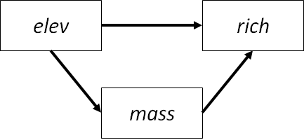
In their study, the authors were interested in the controls of on plant species' density in Finnish meadows. In this worked example, we will consider only elevation and total biomass in their effects on density, plus an effect of elevation on biomass:
Moreover, they repeated their observations in two treatments: grazed and ungrazed meadows. Grazing will serve as the grouping variable for our multigroup analysis.
The data are included in *piecewiseSEM* so let's load it:
```{r}
data(meadows)
```
First, let's construct the "free" model in *lavaan*:
```{r}
jutila_model <- '
rich ~ elev + mass
mass ~ elev
'
jutila_lavaan <- sem(jutila_model, meadows, group = "grazed")
summary(jutila_lavaan)
```
In this example, the model fit can't be determined because the model is saturated (df = 0). This is key moving forward because constraining paths will free up degrees of freedom with which to evaluate model fit.
Let's begin by constraining all paths:
```{r}
jutila_lavaan2 <- sem(jutila_model, meadows, group = "grazed", group.equal = c("intercepts", "regressions"))
summary(jutila_lavaan2)
anova(jutila_lavaan2)
```
The model is significantly different from the unconstrained model we fit previously, implying that some paths could be constrained. Moreover, by constraining the coefficients, we now have 5 degrees of freedom to evaluate model fit. However, it is a poor fit, implying that some path coefficients must vary among groups.
The next step is to sequentially relax and constrain paths:
```{r}
jutila_model2 <- '
rich ~ elev + mass
mass ~ c("b1", "b1") * elev
'
jutila_lavaan3 <- sem(jutila_model2, meadows, group = "grazed")
anova(jutila_lavaan, jutila_lavaan3)
```
The model is still a poor fit, and it is significantly different from the "free" model. In this case, we would conclude that the $elev -> mass$ path should not be constrained.
Let's repeat for the next two paths:
```{r}
# elev -> rich
jutila_model3 <- '
rich ~ c("b2", "b2") * elev + mass
mass ~ elev
'
jutila_lavaan4 <- sem(jutila_model3, meadows, group = "grazed")
anova(jutila_lavaan, jutila_lavaan4)
# mass -> rich
jutila_model4 <- '
rich ~ elev + c("b3", "b3") * mass
mass ~ elev
'
jutila_lavaan5 <- sem(jutila_model4, meadows, group = "grazed")
anova(jutila_lavaan, jutila_lavaan5)
```
Of these two paths, it seems the first: $elev -> rich$, is not significantly different from the "free" model, implying that this path could be constrained. Oppositely, it seems the significant difference between the "free" model and one in which the $mass -> rich$ path is constrained is not supported
Let's check the fit of the model with the one constrait on $elev -> rich$:
```{r}
summary(jutila_lavaan4)
```
Now the model fits the data well ($P = 0.330$), and we have, through an iterative procedure of imposing and relaxing constraints, determined which paths differ among groups ($elev -> mass$, $mass -> rich$) and which do *not* ($elev -> rich$).
Now let's confirm this by fitting the model in *piecewiseSEM*:
```{r}
jutila_psem <- psem(
lm(rich ~ elev + mass, meadows),
lm(mass ~ elev, meadows)
)
multigroup(jutila_psem, group = "grazed")
```
As in our analysis in *lavaan*, the `multigroup` function has identified the $elev -> rich$ path as the only one in which coefficients do not differ among groups. Thus, in the output, that coefficient is the same between groups; otherwise, the coefficients vary depending on whether the meadows is grazed or ungrazed. Moreover, it seems some of the paths differ in their statistical significance: the $rich -> mass$ is not significant in the grazed meadows, but is significant in the ungrazed meadows. So not only do the coefficients differ, but the model structure as well!
You'll note that the *piecewiseSEM* output does not return a goodness-of-fit test because the model is saturated (i.e., no missing paths). While constraints are incorporated in terms of offsets (i.e., fixing model coefficients), unlike global estimation, this does not provide new information with which to test goodness-of-fit. This is a limitation of local estimation that extends beyond multigroup modeling to any piecewise model.
To draw inference about the study system, we would say that two paths differ among groups and one path does not. We would then report the two path models parameterized using the coefficient output (with the $elev -> rich$ path having the same coefficient in both groups). We would report that richness is affected by elevation and biomass under ungrazed conditions, but not under grazed conditions, where only elevation directly influences richness.
## References
Grace, J. B., & Jutila, H. (1999). The relationship between species density and community biomass in grazed and ungrazed coastal meadows. Oikos, 398-408.