-
Notifications
You must be signed in to change notification settings - Fork 3
/
analysis_plan.Rmd
453 lines (307 loc) · 17.2 KB
/
analysis_plan.Rmd
1
2
3
4
5
6
7
8
9
10
11
12
13
14
15
16
17
18
19
20
21
22
23
24
25
26
27
28
29
30
31
32
33
34
35
36
37
38
39
40
41
42
43
44
45
46
47
48
49
50
51
52
53
54
55
56
57
58
59
60
61
62
63
64
65
66
67
68
69
70
71
72
73
74
75
76
77
78
79
80
81
82
83
84
85
86
87
88
89
90
91
92
93
94
95
96
97
98
99
100
101
102
103
104
105
106
107
108
109
110
111
112
113
114
115
116
117
118
119
120
121
122
123
124
125
126
127
128
129
130
131
132
133
134
135
136
137
138
139
140
141
142
143
144
145
146
147
148
149
150
151
152
153
154
155
156
157
158
159
160
161
162
163
164
165
166
167
168
169
170
171
172
173
174
175
176
177
178
179
180
181
182
183
184
185
186
187
188
189
190
191
192
193
194
195
196
197
198
199
200
201
202
203
204
205
206
207
208
209
210
211
212
213
214
215
216
217
218
219
220
221
222
223
224
225
226
227
228
229
230
231
232
233
234
235
236
237
238
239
240
241
242
243
244
245
246
247
248
249
250
251
252
253
254
255
256
257
258
259
260
261
262
263
264
265
266
267
268
269
270
271
272
273
274
275
276
277
278
279
280
281
282
283
284
285
286
287
288
289
290
291
292
293
294
295
296
297
298
299
300
301
302
303
304
305
306
307
308
309
310
311
312
313
314
315
316
317
318
319
320
321
322
323
324
325
326
327
328
329
330
331
332
333
334
335
336
337
338
339
340
341
342
343
344
345
346
347
348
349
350
351
352
353
354
355
356
357
358
359
360
361
362
363
364
365
366
367
368
369
370
371
372
373
374
375
376
377
378
379
380
381
382
383
384
385
386
387
388
389
390
391
392
393
394
395
396
397
398
399
400
401
402
403
404
405
406
407
408
409
410
411
412
413
414
415
416
417
418
419
420
421
422
423
424
425
426
427
428
429
430
431
432
433
434
435
436
437
438
439
440
441
442
443
444
445
446
447
448
449
450
451
452
---
title: "QGT-Columbia-analysis-plan"
author: "Hae Kyung Im"
contributors: "Owen Melia, Yanyu Liang, Tyson Miller"
date: "2020-06-10"
output: workflowr::wflow_html
editor_options:
chunk_output_type: console
---
## Set up
Linux is the operating system of choice to run bioinformatics software. We are offering two options
- Option 1: full setup, recommended for the linux-savvy with full setup
- Option 2: pre-installed RStudio in Google cloud, recommended for people less familiar with linux
The latest version of the analysis plan markdown document that generated this page is on [github here](https://github.com/hakyimlab/QGT-Columbia-HKI/blob/master/analysis/analysis_plan.Rmd)
rendered [here as an html page](https://hakyimlab.github.io/QGT-Columbia-HKI/analysis_plan.html)
# Option 1
- [ ] install anaconda/miniconda
- [ ] define imlabtools conda environment [how to here](https://github.com/hakyimlab/MetaXcan/blob/master/README.md#example-conda-environment-setup), which will install all the python modules needed for this analysis session
- [ ] download data and software [from Box](https://uchicago.box.com/s/zhapf2zfxcpj7thvq4sjnqale3emleum).
This will have copies of all the software repositories and the models
- [x] download software (copies of the repos are already included in the course folder QCT-Columbia-HKI/repos/)
- download metaxcan repo
- download torus repo
- download fastenloc repo
- download TMWR repo
- [x] download prediction models from predictdb.org (a few models are included in the course folder QCT-Columbia-HKI/repos/)
- [ ] install R/RStudio/tidyverse package
- [ ] (optional) install workflowr package in R
- [ ] git clone https://github.com/hakyimlab/QGT-Columbia-HKI.git
- [ ] start Rstudio (if you installed workflowr, you can just open the QGT-Columbia-HKI.Rproj)
# Option 2
- [ ] claim your Rstudio server IP address and get the username and password [here](https://drive.google.com/file/d/1RNeOrOfORiS0PFuv4r0d6E2N5XE7I1tV/view?usp=sharing)
- [ ] connect to the Rstudio server using the url you claimed (http://xxx.xxx.xxx.xxx:8787) using a web browser
- [ ] log into the server using the username and password of the server you claimed
# Both options
## Summary of analysis plan
- predict whole blood expression
- check how well the prediction works with GEUVADIS expression data
- run association between predicted expression and a simulated phenotype
- calculate association between expression levels and coronary artery disease risk using s-predixcan
- fine-map the coronary artery disease gwas results using torus
- calculate colocalization probability using fastenloc
- run transcriptome-wide mendelian randomization in one locus of interestgi
## Initial remarks
- We ask you to actively participate in today's hands on activities. **Notice that we may ask you to share your screen for pedagogic purposes.**
- As you run the analysis and programs, we ask you to **respond the questions in [this document](https://drive.google.com/file/d/1RNeOrOfORiS0PFuv4r0d6E2N5XE7I1tV/view?usp=sharing).**
Find the tab with your name and fill out the questions as you go along.
- You are welcome to check other people's answers as guidelines but please make sure you write down your own answers.
- If you have any concerns about this, please ask me or one of the TAs for assistance. We are here to help you learn.
## Preliminary definitions
- [ ] Go to the terminal tab on the RStudio server and update the analysis document to the most recent version. The commands are shown below. Copy the text (without the lines with apostrophes: ```), paste them to the *terminal*, and hit enter.
```{bash eval=FALSE}
PRE="/home/student/"
cd $PRE/lab/
git pull
```
- [ ] activate the the imlabtools environment, which will make sure all the necessary python modules are available to the software we will be running.
```{bash, eval=FALSE}
conda activate imlabtools
```
**Reminder: the bash chunks need to be copy-pasted to the terminal, not performed within the chunk.**
- [ ] execute the following chunk (you can use the green arrow below to the right)
```{r preliminary definitions, eval=FALSE}
suppressPackageStartupMessages(library(tidyverse))
```
- [ ] define some variables to access the data more easily within the R session. Run the following r chunk
```{r preliminaries, eval=FALSE}
print(getwd())
lab="/home/student/lab"
CODE=glue::glue("{lab}/code")
source(glue::glue("{CODE}/load_data_functions.R"))
source(glue::glue("{CODE}/plotting_utils_functions.R"))
PRE="/home/student/QGT-Columbia-HKI"
MODEL=glue::glue("{PRE}/models")
DATA=glue::glue("{PRE}/data")
RESULTS=glue::glue("{PRE}/results")
METAXCAN=glue::glue("{PRE}/repos/MetaXcan-master/software")
FASTENLOC=glue::glue("{PRE}/repos/fastenloc-master")
TORUS=glue::glue("{PRE}/repos/torus-master")
TWMR=glue::glue("{PRE}/repos/TWMR-master")
# This is a reference table we'll use a lot throughout the lab. It contains information about the genes.
gencode_df = load_gencode_df()
```
- [ ] define some variables to access the data more easily in the terminal. Run the following bash chunk. You will need to copy and paste the following chunk in the terminal
```{bash folder name variables, eval=FALSE}
export PRE="/home/student/QGT-Columbia-HKI"
export LAB="/home/student/lab"
export CODE=$LAB/code
export DATA=$PRE/data
export MODEL=$PRE/models
export RESULTS=$PRE/results
export METAXCAN=$PRE/repos/MetaXcan-master/software
export TWMR=$PRE/repos/TWMR-master
```
# Transcriptome-wide association methods
## predict expression
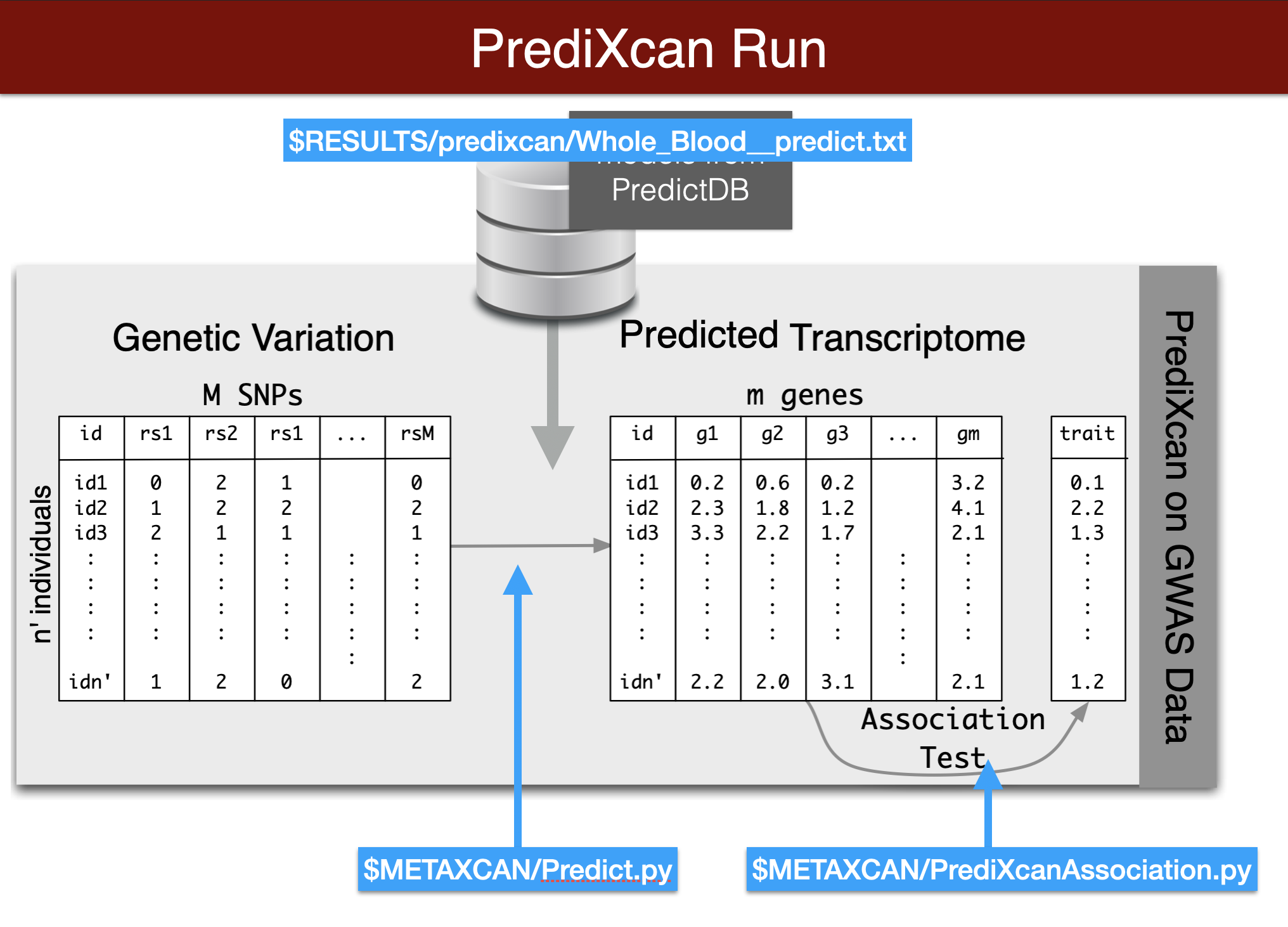
- We will predict expression of genes in whole blood using the Predict.py code in the METAXCAN folder.
- Prediction models are located in the MODEL folder. Additional models for different tissues and transcriptome studies can be downloaded from [predictdb.org](http://predictdb.org)
- Remember you need to copy and paste this code chunk into the terminal to run it. Also make sure you activated the imlabtools environment which has all the necessary python modules.
- Make sure all the paths and file names are correct
- This run should take about one minute.
- [ ] copy and paste the following block to the terminal and hit enter
```{bash predict genetic component of expression, eval=FALSE}
printf "Predict expression\n\n"
python3 $METAXCAN/Predict.py \
--model_db_path $PRE/models/gtex_v8_en/en_Whole_Blood.db \
--vcf_genotypes $DATA/predixcan/genotype/filtered.vcf.gz \
--vcf_mode genotyped \
--variant_mapping $DATA/predixcan/gtex_v8_eur_filtered_maf0.01_monoallelic_variants.txt.gz id rsid \
--on_the_fly_mapping METADATA "chr{}_{}_{}_{}_b38" \
--prediction_output $RESULTS/predixcan/Whole_Blood__predict.txt \
--prediction_summary_output $RESULTS/predixcan/Whole_Blood__summary.txt \
--verbosity 9 \
--throw
```
- [ ] check predicted values (run the following chunk using the green arrow)
```{r check prediction performance, eval=FALSE}
prediction_fp = glue::glue("{RESULTS}/predixcan/Whole_Blood__predict.txt")
## Read the Predict.py output into a dataframe. This function reorganizes the data and adds gene names.
predicted_expression = load_predicted_expression(prediction_fp, gencode_df)
head(predicted_expression)
## read summary of prediction, number of SNPs per gene, cross validated prediction performance
prediction_summary = load_prediction_summary(glue::glue("{RESULTS}/predixcan/Whole_Blood__summary.txt"), gencode_df)
## number of genes with a prediction model
dim(prediction_summary)
head(prediction_summary)
print("distribution of prediction performance r2")
summary(prediction_summary$pred_perf_r2)
```
## assess prediction performance (optional)
```{r assess prediction performance, eval=FALSE}
## download and read observed expression data from GEUVADIS
## from https://uchicago.box.com/s/4y7xle5l0pnq9d1fwmthe2ewhogrnlrv
## Remove the version number from the gene_id's (ENSG000XXX.ver)
head(predicted_expression)
## merge predicted expression with observed expression data (by IID and gene)
## plot observes vs predicted expressioni for
## ERAP1 (ENSG00000164307)
## PEX6 (ENSG00000124587)
## calculate spearman correlation for all genes
## what's the best performing gene?
```
## run association with a simulated phenotype
$Y = \sum_k T_k \beta_k + \epsilon$
with random effects $\beta_k \sim (1-\pi)\cdot \delta_0 + \pi\cdot N(0,1)$
```{bash run predixcan association, eval=FALSE}
export PHENO="sim.spike_n_slab_0.01_pve0.1"
printf "association\n\n"
python3 $METAXCAN/PrediXcanAssociation.py \
--expression_file $RESULTS/predixcan/Whole_Blood__predict.txt \
--input_phenos_file $DATA/predixcan/phenotype/$PHENO.txt \
--input_phenos_column pheno \
--output $RESULTS/predixcan/$PHENO/Whole_Blood__association.txt \
--verbosity 9 \
--throw
```
More predicted phenotypes can be [downloaded from here](https://uchicago.box.com/s/xxzuzjamscpc365ui9ge98le0qwy11wz). The naming of the phenotypes provides information about the genic architecture: the number after pve is the proportion of variance of Y explained by the genetic component of expression. The number after spike_n_slab represents the probability that a gene is causal $\pi$(i.e. prob $\beta \ne 0$)
## read association results
```{r read predixcan association results, eval=FALSE}
## read association results
PHENO="sim.spike_n_slab_0.01_pve0.1"
predixcan_association = load_predixcan_association(glue::glue("{RESULTS}/predixcan/{PHENO}/Whole_Blood__association.txt"),
gencode_df)
## take a look at the results
dim(predixcan_association)
predixcan_association %>% arrange(pvalue) %>% head
predixcan_association %>% arrange(pvalue) %>% ggplot(aes(pvalue)) + geom_histogram(bins=20)
## compare distribution against the null (uniform)
gg_qqplot(predixcan_association$pvalue, max_yval = 40)
```
## compare estimated effects with true effect sizes
```{r read true effect sizes, eval=FALSE}
truebetas = load_truebetas(glue::glue("{DATA}/predixcan/phenotype/gene-effects/{PHENO}.txt"), gencode_df)
betas = (predixcan_association %>%
inner_join(truebetas,by=c("gene"="gene_id")) %>%
select(c('estimated_beta'='effect',
'true_beta'='effect_size',
'pvalue',
'gene_id'='gene',
'gene_name'='gene_name.x',
'region_id'='region_id.x')))
betas %>% arrange(pvalue) %>% head
## do you see examples of potential LD contamination?
betas %>% ggplot(aes(predicted_beta, true_beta))+geom_point()+geom_abline()
```
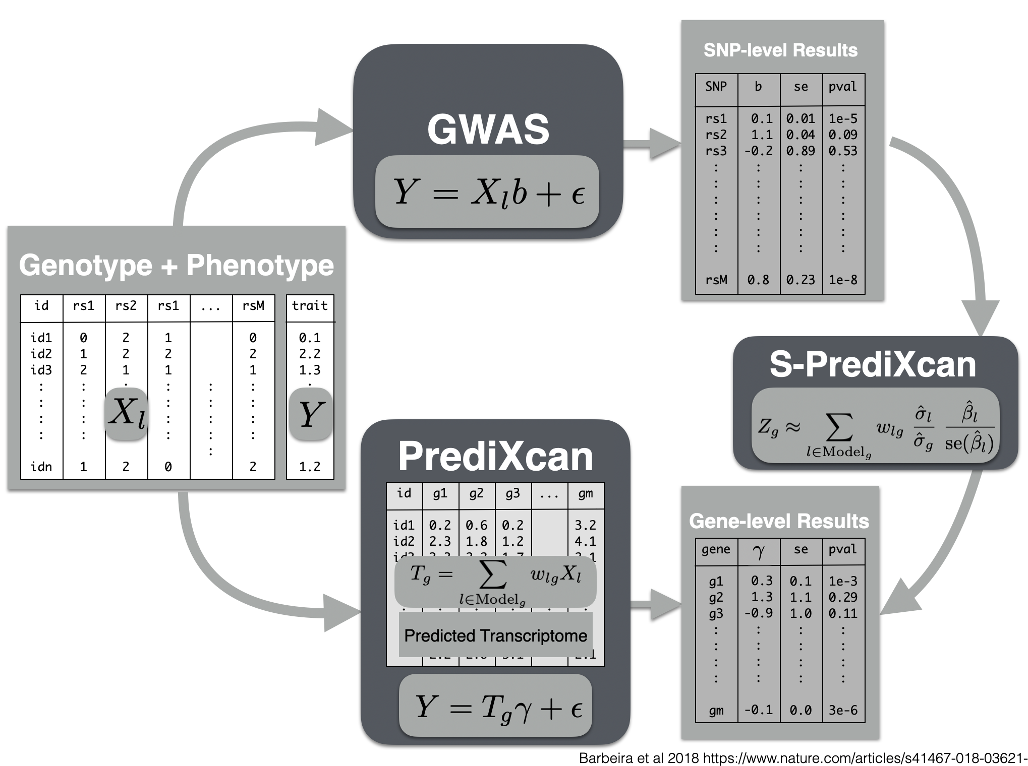
# Summary PrediXcan
Now we will use the summary results from a GWAS of coronary artery disease to calculate the association between the genetic component of the expression of genes and coronary artery disease risk. We will use the SPrediXcan.py.
- harmonized and imputed GWAS result for coronary artery disease is available in $PRE/spredixcan/data/
## run s-predixcan
```{bash run s-predixcan, eval=FALSE}
python $METAXCAN/SPrediXcan.py \
--gwas_file $DATA/spredixcan/imputed_CARDIoGRAM_C4D_CAD_ADDITIVE.txt.gz \
--snp_column panel_variant_id --effect_allele_column effect_allele --non_effect_allele_column non_effect_allele --zscore_column zscore \
--model_db_path $MODEL/gtex_v8_mashr/mashr_Whole_Blood.db \
--covariance $MODEL/gtex_v8_mashr/mashr_Whole_Blood.txt.gz \
--keep_non_rsid --additional_output --model_db_snp_key varID \
--throw \
--output_file $RESULTS/spredixcan/eqtl/CARDIoGRAM_C4D_CAD_ADDITIVE__PM__Whole_Blood.csv
```
## plot and interpret s-predixcan results
```{r analyze s-predixcan results, eval=FALSE}
spredixcan_association = load_spredixcan_association(glue::glue("{RESULTS}/spredixcan/eqtl/CARDIoGRAM_C4D_CAD_ADDITIVE__PM__Whole_Blood.csv"), gencode_df)
dim(spredixcan_association)
spredixcan_association %>% arrange(pvalue) %>% head
spredixcan_association %>% arrange(pvalue) %>% ggplot(aes(pvalue)) + geom_histogram(bins=20)
gg_qqplot(spredixcan_association$pvalue)
```
- [ ] SORT1, considered to be a causal gene for LDL cholesterol and as a consequence of coronary artery disease, is not found here. Why? (tissue)
## Exercise
- [ ] run s-predixcan with liver model, do you find SORT1? Is it significant?
- [ ] compare zscores in liver and whole blood.
## run multixcan (optional)
- multixcan aggregates information across multiple tissues to boost the power to detect association. It was developed movivated by the fact that eQTLs are shared across multiple tissues, i.e. many genetic variants that regulate expression are common across tissues.
```{bash run multixcan, eval=FALSE}
python $METAXCAN/SMulTiXcan.py \
--models_folder $MODEL/gtex_v8_mashr \
--models_name_pattern "mashr_(.*).db" \
--snp_covariance $MODEL/gtex_v8_expression_mashr_snp_smultixcan_covariance.txt.gz \
--metaxcan_folder $RESULTS/spredixcan/eqtl/ \
--metaxcan_filter "CARDIoGRAM_C4D_CAD_ADDITIVE__PM__(.*).csv" \
--metaxcan_file_name_parse_pattern "(.*)__PM__(.*).csv" \
--gwas_file $DATA/spredixcan/imputed_CARDIoGRAM_C4D_CAD_ADDITIVE.txt.gz \
--snp_column panel_variant_id --effect_allele_column effect_allele --non_effect_allele_column non_effect_allele --zscore_column zscore --keep_non_rsid --model_db_snp_key varID \
--cutoff_condition_number 30 \
--verbosity 7 \
--throw \
--output $RESULTS/smultixcan/eqtl/CARDIoGRAM_C4D_CAD_ADDITIVE_smultixcan.txt
```
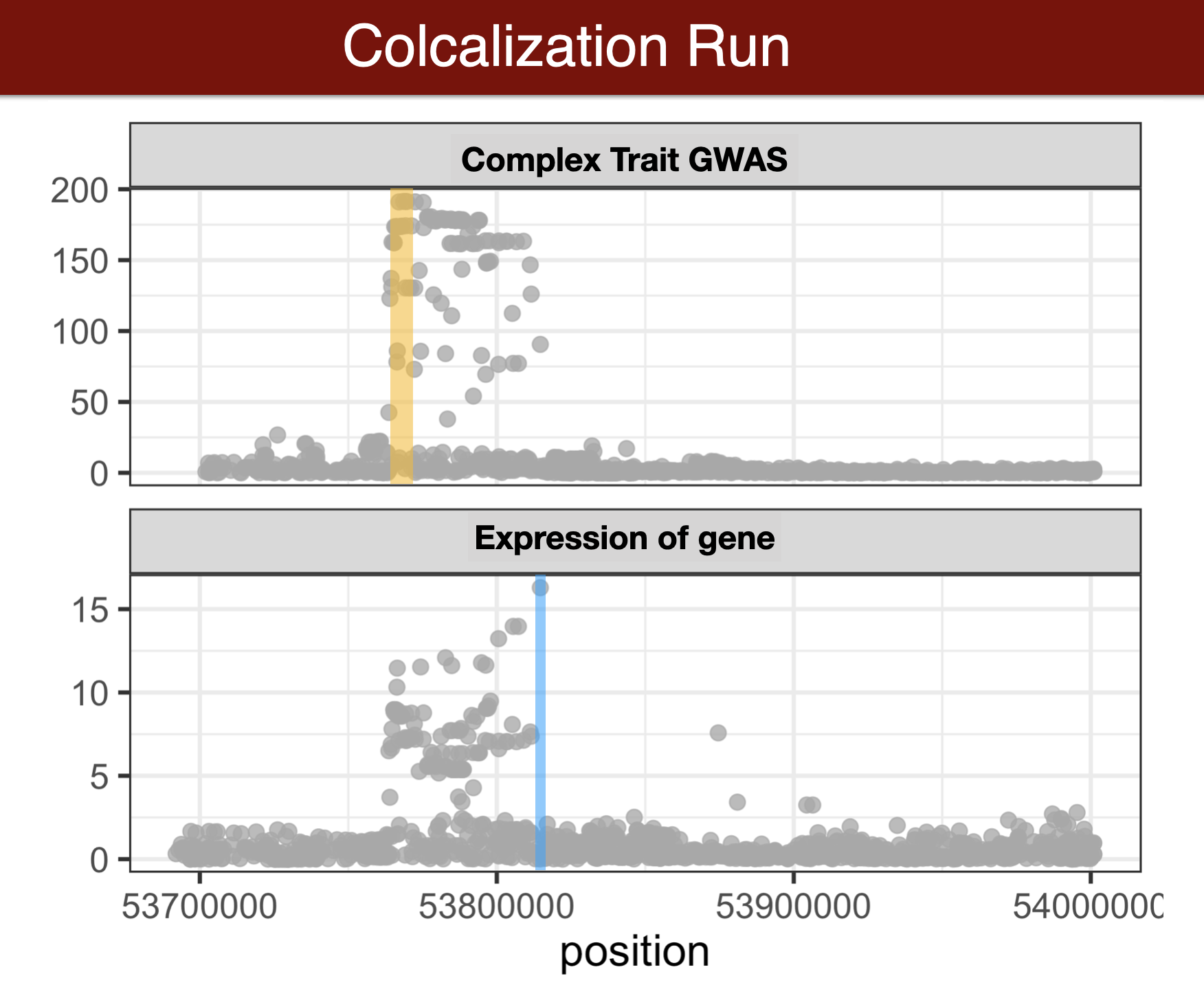
# Colocalization methods
- Colocalization methods seek to estimate the probability that the complex trait and expression causal variants are the same. We favor methods that calculate the probability of causality for each trait (posterior inclusion probability), called fine-mapping methods. Here we use torus for fine-mapping and fastENLOC for colocalization.
## GWAS summary statistics to torus format
- the following code will format GWAS summary statistics into a format that the fine-mapping method torus can understand.
- we precalculated this for you so there is no need to recalculate
```{bash, eval=FALSE}
## notice that the GWAS results are in hg38
python $CODE/gwas_to_torus_zscore.py \
-input_gwas $DATA/spredixcan/imputed_CARDIoGRAM_C4D_CAD_ADDITIVE.txt.gz \
-input_ld_regions $DATA/spredixcan/eur_ld_hg38.txt.gz \
-output_fp $DATA/fastenloc/CARDIoGRAM_C4D_CAD_ADDITIVE.zval.gz
```
## fine-map GWAS results
- We will run torus due to time limitation but ideally we would like to run a method that allows multiple causal variants per locus, such as DAP-G or SusieR.
- torus has been precompiled and placed within the PATH
```{bash run torus, eval=FALSE}
export TORUSOFT=torus
$TORUSOFT -d $PRE/data/fastenloc/CARDIoGRAM_C4D_CAD_ADDITIVE.zval.gz --load_zval -dump_pip $PRE/data/fastenloc/CARDIoGRAM_C4D_CAD_ADDITIVE.gwas.pip
cd $PRE/data/fastenloc
gzip CARDIoGRAM_C4D_CAD_ADDITIVE.gwas.pip
cd $PRE
```
We can take a quick look at the z-values and finemapping PIPs:
```{bash, eval=FALSE}
cd $PRE/data/fastenloc
zless CARDIoGRAM_C4D_CAD_ADDITIVE.zval.gz
zless CARDIoGRAM_C4D_CAD_ADDITIVE.gwas.pip.gz
```
## calculate colocalization with fastENLOC
```{bash run fastENLOC, eval=FALSE}
## check out tutorial https://github.com/xqwen/fastenloc/tree/master/tutorial
export eqtl_annotation_gzipped=$PRE/data/fastenloc/FASTENLOC-gtex_v8.eqtl_annot.vcf.gz
export gwas_data_gzipped=$PRE/data/fastenloc/CARDIoGRAM_C4D_CAD_ADDITIVE.gwas.pip.gz
export TISSUE=Whole_Blood
export FASTENLOCSOFT=fastenloc
##export FASTENLOCSOFT=/Users/owenmelia/projects/finemapping_bin/src/fastenloc/src/fastenloc
mkdir $RESULTS/fastenloc/
cd $RESULTS/fastenloc/
$FASTENLOCSOFT -eqtl $eqtl_annotation_gzipped -gwas $gwas_data_gzipped -t $TISSUE
#[-total_variants total_snp] [-thread n] [-prefix prefix_name] [-s shrinkage]
```
## analyze results
```{r analyze torus results, eval=FALSE}
## optional - compare with s-predixcan results
fastenloc_results = load_fastenloc_coloc_result(glue::glue("{RESULTS}/fastenloc/enloc.sig.out"))
spredixcan_and_fastenloc = inner_join(spredixcan_association, fastenloc_results, by=c('gene'='Signal'))
ggplot(spredixcan_and_fastenloc, aes(RCP, -log10(pvalue))) + geom_point()
## which genes are both colocalized (rcp>0.10) and significantly associated (pvalue<0.05/number of tests)
```
----------
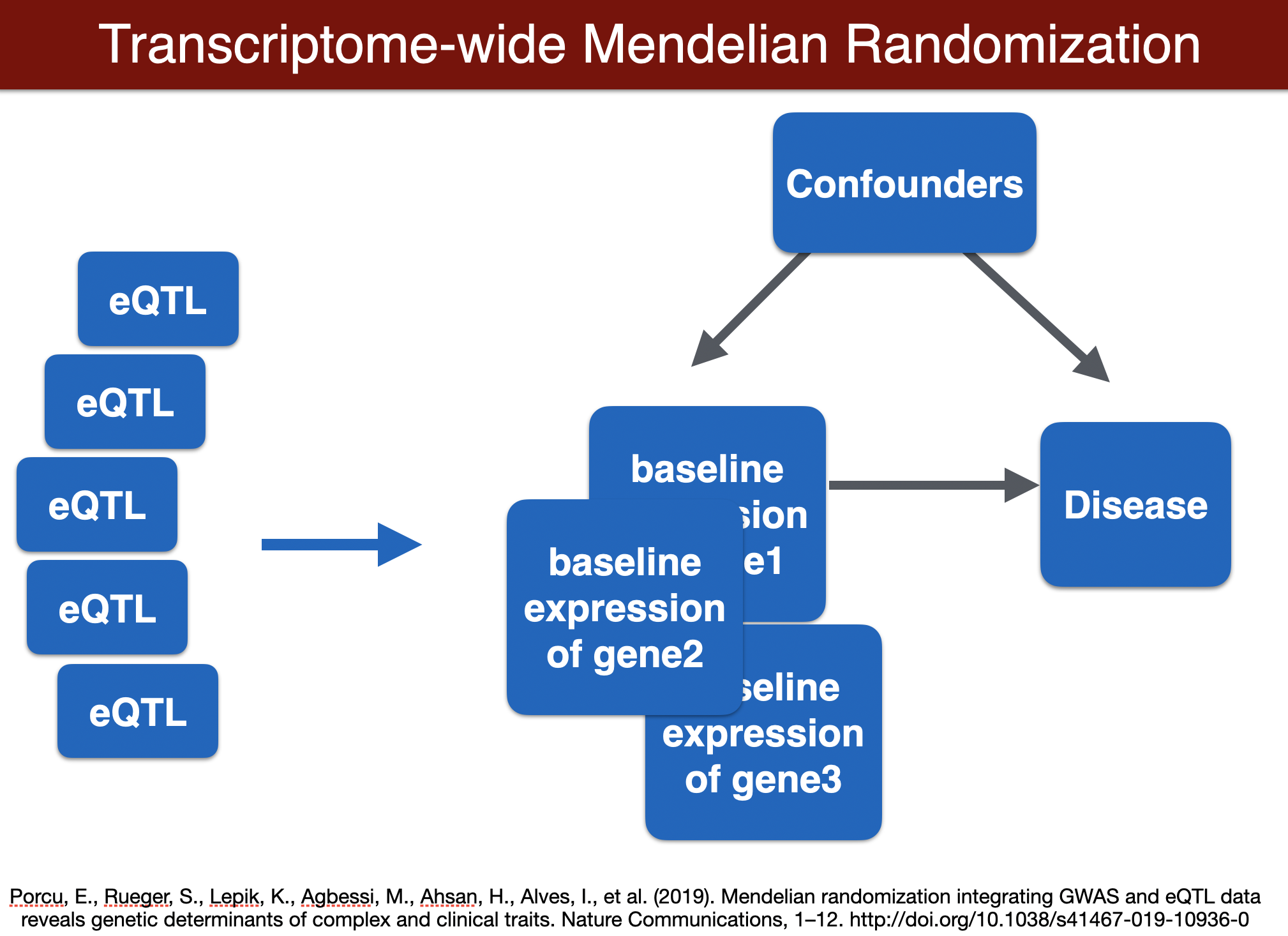
# Mendelian randomization methods
## run TWMR (for a locus)
```{bash run TWMR, eval=FALSE}
GENE=ENSG00000002919
cd $TWMR
R < $TWMR/MR.R --no-save $GENE
cd $PRE
## output: /home/student/QGT-Columbia-HKI/repos/TWMR-master/ENSG00000002919.alpha
```
```{r run TWMR, eval=FALSE}
# Load the 'analyseMR' function
source(glue::glue("{CODE}/TWMR_script.R"))
# Collect the list of genes available to run
gene_lst <- list.files(TWMR)
gene_lst <- gene_lst[str_detect(gene_lst, "ENS.*")]
gene_lst <- (gsub("\\..*", "", gene_lst) %>% unique)
# Set the gene and run. The function writes output to a file.
for (gene in gene_lst) {
analyseMR(gene, TWMR)
}
```
```{r analyze TWMR results, eval=FALSE}
twmr_results <- load_twmr_results(TWMR, gencode_df)
```