In this module, we would explore concepts related to data warehouse. The choice of data warehouse for this module is GCS BigQuery.
- OLAP vs OLTP
- Data Warehouse
- Partitioning vs Clustering
- BigQuery Best Practice
- BigQuery Internals
- References
There are 2 types of database architectures that help us store and analyze business data, namely OLAP (online analytical processing) and OLTP (online transaction processing).
The key differences can be summarize to the following table
| OLTP | OLAP | |
|---|---|---|
| Purpose | Control and run essential business operations in real time | Plan, solve problems, support decisions, discover hidden insights |
| Data source | Real-time and transactional data from a single source | Historical and aggregated data from multiple sources |
| Operations | Based on INSERT, UPDATE, DELETE commands | Based on SELECT commands to aggregate data for reporting |
| Data updates | Short, fast updates initiated by user | Data periodically refreshed with scheduled, long-running batch jobs |
| Volume of data | Smaller storage requirements. Think gigabytes (GB). | Large storage requirements. Think terabytes (TB) and petabytes (PB). |
| Response time | Shorter response times, typically in milliseconds | Longer response times, typically in seconds or minutes |
| Backup and recovery | Regular backups required to ensure business continuity and meet legal and governance requirements | Lost data can be reloaded from OLTP database as needed in lieu of regular backups |
| Database design | Normalized databases for efficiency | Denormalized databases for analysis |
| Example | MySQL, PostgreSQL, Oracle Database | Amazon Redshift, Google BigQuery, Snowflake |
Note
Normalized databases reduce data redundancy and ensure data integrity by dividing data into multiple, connected tables based on specific rules (normal forms).
Note
Denormalized databases improve query performance at the expense of some data redundancy by combining data from multiple tables into a single table or flattens data structures.
Data warehouse uses a ETL (Extract-Transform-Load) process unlike datalake which uses a ELT (Extract-Load-Transform) process.
In order to automate the loading of NY taxi data from NY Taxi record page to Google Cloud Storage, I had created a data ingestion script which utilizes wget and Cloud Storage Python API. The script can be run with the following command:
python3 data_ingestion_to_gcs.py [--year YEAR] [--color COLOR] [--bucket BUCKET] [--blob BLOB]Google BigQuery allows querying data stored outside of BigQuery. External tables are similar to standard BigQuery tables, in that these tables store their metadata and schema in BigQuery storage. However, their data resides in an external source. In our case, we would be querying from Google Cloud Storage.
To create external table from GCS path, we could execute the following sql statement
-- Creating external table referring to gcs path
CREATE OR REPLACE EXTERNAL TABLE `taxi-rides-ny.nytaxi.external_yellow_tripdata`
OPTIONS (
  format = 'PARQUET',
  uris = ['gs://nyc-tl-data/yellow_taxi/yellow_tripdata_2019-*.parquet']
);
You may perform SQL query on the external table.
Note
BQ is unable to determine the number of rows for external table.
To convert external table to internal table, we could execute the following sql statement.
-- Create a non partitioned table from external table
CREATE OR REPLACE TABLE taxi-rides-ny.nytaxi.yellow_tripdata_non_partitoned AS
SELECT * FROM taxi-rides-ny.nytaxi.external_yellow_tripdata;Partitioning table improve query performance and control costs by reducing the number of bytes read by a query. If a query uses a qualifying filter on the value of the partitioning column, BigQuery can scan the partitions that match the filter and skip the remaining partitions.
In a partitioned table, data is stored in physical blocks, each of which holds one partition of data. Each partitioned table maintains various metadata about the sort properties across all operations that modify it.
We could partition a table by specifying a partition column which is used to segment the table. Query below shows an example to partition an external table.
-- Create a partitioned table from external table
CREATE OR REPLACE TABLE taxi-rides-ny.nytaxi.yellow_tripdata_partitoned
PARTITION BY
  DATE(tpep_pickup_datetime) AS
SELECT * FROM taxi-rides-ny.nytaxi.external_yellow_tripdata;
There are various ways to partition a table.
- Integer range partitioning - partition a table based on ranges of values in a specific INTEGER column.
CREATE TABLE mydataset.newtable (customer_id INT64, date1 DATE)
PARTITION BY
  RANGE_BUCKET(customer_id, GENERATE_ARRAY(0, 100, 10))
  OPTIONS (
    require_partition_filter = TRUE);
example taken from Google BigQuery Documentation Creating partitioned tables
- Time-unit column partitioning - partition a table on a DATE,TIMESTAMP, or DATETIME column in the table.
CREATE TABLE
  mydataset.newtable (transaction_id INT64, transaction_date DATE)
PARTITION BY
  transaction_date
  OPTIONS (
    partition_expiration_days = 3,
    require_partition_filter = TRUE);
example taken from Google BigQuery Documentation Creating partitioned tables
- Ingestion time partitioning ( _PARTITIONDATE) - automatically assigns rows to partitions based on the time when BigQuery ingests the data.
CREATE TABLE
  mydataset.newtable (transaction_id INT64)
PARTITION BY
  _PARTITIONDATE
  OPTIONS (
    partition_expiration_days = 3,
    require_partition_filter = TRUE);
example taken from Google BigQuery Documentation Creating partitioned tables
Clustered tables are tables that have a user-defined column sort order using clustered columns. Order of the column is important as it determines the sort order of the data.
Query below shows an example to partition and cluster an external table.
-- Creating a partition and cluster table
CREATE OR REPLACE TABLE taxi-rides-ny.nytaxi.yellow_tripdata_partitoned_clustered
PARTITION BY DATE(tpep_pickup_datetime)
CLUSTER BY VendorID AS
SELECT * FROM taxi-rides-ny.nytaxi.external_yellow_tripdata;It is generally better to only use partitioning unless the following scenarios are met
- Partitioning results in a small amount of data per partition (approximately less than 1 GB)
- Partitioning results in a large number of partitions beyond the limits on partitioned tables (4000 partitions is the limit)
- Partitioning results in your mutation operations modifying the majority of partitions in the table frequently (for example, every few minutes)
-
Cost Reduction
- Avoid SELECT *
- Price your queries before running them
- Use clustered or partitioned tables
- Use streaming inserts with caution
- Materialize query results in stages
-
Query Performance
- Filter on partitioned columns
- Denormalizing data
- Use nested or repeated columns
- Use external data sources appropriately
- Don't use it, in case u want a high query performance
- Reduce data before using a JOIN
- Do not treat WITH clauses as prepared statements
- Avoid oversharding tables
- Avoid JavaScript user-defined functions
- Use approximate aggregation functions
- Order Last, for query operations to maximize performance
- Optimize join patterns
- As a best practice, place the table with the largest number of rows first, followed by the table with the fewest rows, and then place the remaining tables by decreasing size.
The internal working is explained in the blog post BigQuery under the hood.
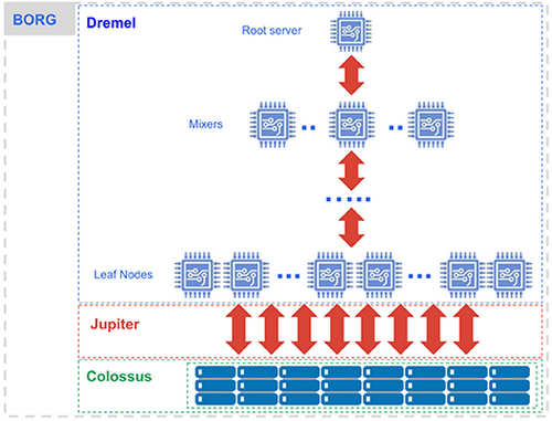
BigQuery requests are powered by the Dremel query engine. Dremel turns your SQL query into an execution tree. The leaves of the tree it calls ‘slots’, and do the heavy lifting of reading the data from Colossus and doing any computation necessary. The branches of the tree are ‘mixers’, which perform the aggregation. The mixers and slots are all run by Borg, which doles out hardware resources.
BigQuery leverages the ColumnIO columnar storage format and compression algorithm to store data in Colossus in the most optimal way for reading large amounts of structured data.
Besides obvious needs for resource coordination and compute resources, Big Data workloads are often throttled by networking throughput, and it is done via Jupyter networking infrastructure.