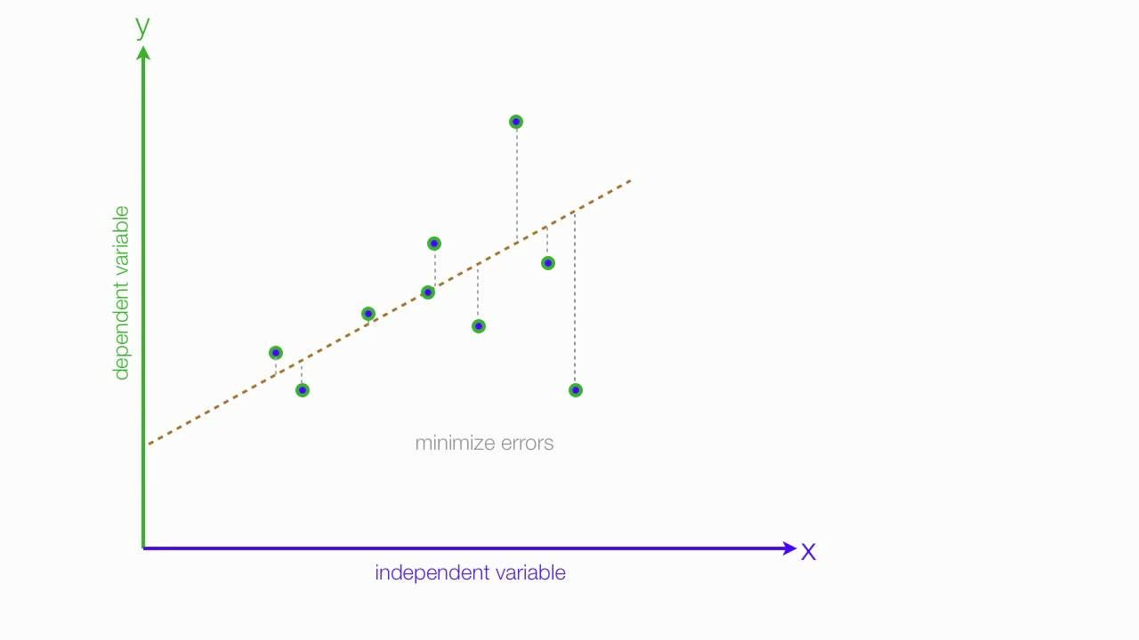
linear_regression.rst

Linear regression

Linear regression is a linear approach to modeling the relationship between a scalar response (or dependent variable) which is continuous and one or more explanatory variables (or independent variables) (Ref.: Wikipedia).

쉽게 설명하면 주어진 데이터를 가장 잘 설명하는 직선 하나를 찾는 것이 Linear regression이다.

I will explain linear regression using a housing price prediction example.

Univariate linear regression

Univariate linear regression is the linear regression with one variable. → 즉, 하나의 설명 변수로 선을 찾는 것이 Univariate linear regression이다.

A below figure describes housing price prediction with univariate linear regression.

Process

A hypothesis function is a prediction model trained by a cost function using training set.

This is a training set example.

• m = The number of training examples (samples)
• x′s = Input variables (Features)
• y′s = Output variables (Target variables)
• (x, y) = One training example
• (x_i, y_i) = i_thtraining example

결론적으로 주어진 데이터로 θ₀ 와 θ₁ 을 찾는 것이다.

Cost function

To find the best parameters, we should minimize costs for training examples. So, we need a cost function to calculate losses between predictions and answers.

centered

Source: towards data science

Idea:

• Choose θ₀, θ₁ so that h_θ(x) is close to y for training samples

• Examples:

  

This is one of the methods called Mean Suqared Error (MSE or L2 loss) for the cost function and the goal is to minimize the squared error function.

Besides the MSE function, there are many cost functions (Link <loss_func>).

결국, 우리의 목적은 이러한 MSE가 최소화가 되도록 θ₀, θ₁ 을 구하는 것이고, 단순히 최적의 θ₁ 을 구하는 방법은 θ₁ = (x^Tx)^− 1x^Ty (수식 이해 안감)를 푸는 것이다. 하지만 데이터가 커짐에 따라 시간 복잡도가 O(n³) 로 증가하여 비효율적이다. 그래서 이러한 문제를 해결하는 방법이 Gradient descent이다.

Gradient descent

Gradient descent is a first-order iterative optimization algorithm for finding the minimum of a function. To find a local minimum of a function using gradient descent, one takes steps proportional to the negative of the gradient (or approximate gradient) of the function at the current point (Ref.: Wikipedia).

즉, Gradient descent는 기존 Weight에 Error function의 미분값을 빼주면서 Weight를 업데이트하는 방법이다.

This is how to update weights using gradient descent for all training dataset:

centered

$\displaystyle w:=w-\eta \nabla Q(w)=w-\eta \sum _{i=1}^{n}\nabla Q_{i}(w)/n,$

Anyway, we talk about all from now step by step.

Idea:

• Make arbitrary function J(θ₀, θ₁)
• Find min_θ0, θ1J(θ₀, θ₁)

Process:

• Start with some θ₀, θ₁
• Keep changing θ₀, θ₁ to reduce J(θ₀, θ₁) until we hopefully end up at a minimum

Types

• Batch gradient descent

  • Each step of gradient descent uses all the training set.

• Stochastic gradient descent (SGD)

  • Each step of gradient descent uses partial of the training set called mini-batch.

• Others (Link <optimization>)

Algorithm

Linear equation movement

In the cost function, a gradient speed can be decided by the learning rate.

Also, we don't need to decrease the learning rate because gradient will be getting smaller in every step.

While being trained, the model can be stuck in a local minimum problem:

Multivariate linear regression

Multivariate linear regression is the linear regression with multi variable.

Features and hypothesis function

Univariate linear regression:

• Features

  Size	Price
  2,104	460
  1,416	232
  1,534	315
  ...	...

• Hypothesis function

  centered

  h_θ(x) = θ₀ + θ₀x

Multiple linear regression:

• Features

  Size	Price	# of rooms	# of floors	Age
  2,104	460	5	1	45
  1,416	232	3	2	40
  1,534	315	3	2	30
  ...	...	...	...	...

• Hypothesis function

  centered

  $h_{\theta}(x) = \displaystyle\sum_{i=0}^{n} \theta_{i}x_{i}\ \ where\ \theta_{i}=weight,\ x_{0}=1$

Gradient descent for multiple variables

Algorithm

Should be update simultaneously!!

Feature scaling

All features have different scale, so we need to make all features are on a similar scale

• Before:

  • A lots of iterations are needed
  • :math:x_{1} = size,(0 - 2000)
  • :math:x_{2} = #ofrooms,(1 - 5)

  

• After:

  • A few interations are nedded
  • $x_{1} = \frac{size}{2000}, (0 - 1)$
  • $x_{2} = \frac{\#\ of\ rooms}{5}, (0.2 - 1)$

  

Types

• Mean normalization

  • $x_{i\_mean} = \frac{x_{i} - average(x_{i})}{range(x_{i})}, (-1 \leq x_{i\_mean} \leq 1)$

• Standardization

  • $x_{i\_std} = \frac{x_{i} - min(x_{i})}{range(x_{i})}, (-1 \leq x_{i\_std} \leq 1)$

Normal equation

• Alternative method to get weight value
• Don’t need iteration

• Method:

  :math:text{For every } n, text{training data } m \ frac{partial J}{partial theta_{n}} = displaystylesum_{i=1}^{m} (theta_{0} + theta_{1}x_{i} + cdots + theta_{1}x_{i}^{n} - y_{i}) \ Rightarrow theta = (X^{T}X)^{-1}X^{T}Y

Gradient descent vs. Normal equation

Gradient descent	Normal equation
Should decide learning rate	Don‘t need to decide learning rate
Many iteration	No iteration
Relatively little calculation	A lot of calculation

Summary

• Linear regression is an regression analysis method by making a regression model with cost function and gradient decent using training set
• Multivariate linear regression can be performed like univariate linear regression

• There are two method for multivariate liner regression

  • Gradient descent
  • Normal equation

• Each method has its own benefit

Reference

• One page summary
• Coursera, Machine Learning