This is a python program that can test and visualize the A* path planning algorithnm to navigate a robot between two points in a 2D map.
- Install python from here
- Install matplotlib from here
- Open the program directory in terminal or command prompt and run the program with the following command:
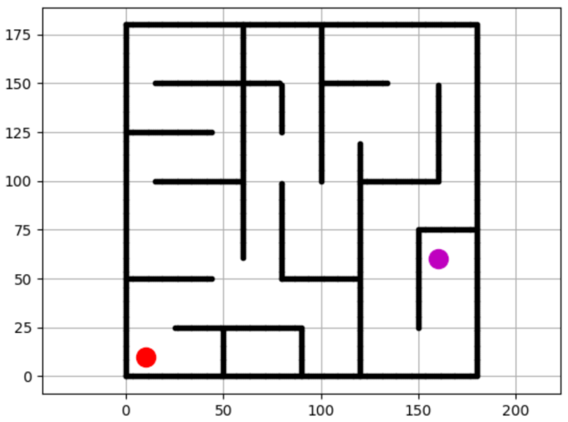
python path_planning_test.pyThe program will initialize the following maze as a 180x180m^2 2D map with a grid size of 1m:
 |
|---|
| Figure 1: A 2D map of a maze |
The red dot shows the start point (-10,-10)m and the magenta dot shows the goal point (160,60)m of the robot. The A* algorithm will search for the shortest path from the start point to the goal point while avoiding obstacles along the way. The robot has a radius of 1m and/
A* is a pathfinding algorithm that can find the shortest path between two nodes in a graph.
A* chooses the path with the minimum value of the function f(n) as defined as follows:
f(n) = g(n) + h(n)
Where:
- n is the next node (Neighbouring node) on the path
- g(n) is the actual cost of the path from the start node to n
- h(n) is the estimated cost of the path from n to
 |
|---|
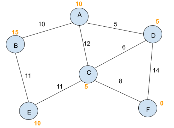
| Figure 2: An example of a weighted graph |
| Source: isaaccomputerscience.org |
The A* algorithm executes the following steps to determine the minimum path between two nodes:
-
Insert all nodes into a set of unvisited nodes called open set
-
Initialize the stored f(n) values of all nodes as Infinity and the address of the previous node of all nodes as None
-
Set the start node as the currently visited node
-
From the current node, choose a neighboring node with the minimum value of f(n) = g(n) + h(n)
- The value of g(n) is determined by the total cost of path from the start node to reach the neighbouring node (Denoted by the black numbers in Figure 1)
- The value of h(n) is determined by the value of a heuristic function that estimates the cost between the neighboring node to the goal node (Denoted by the orange numbers in Figure 1)
- Example of heuristic functions h(n) that can be used are Euclidean distance, Manhattan distance, and Great-circle distance
-
Consider the values of f(n) and the address of the previous node for each neighboring nodes
- If the current f(n) value of a neighboring node is lower than the stored f(n) value of that node store the value f(n) and the previous node of n
- Else, ignore the node n
-
Once all neighbouring nodes n of the current node has been considered, remove the current node from the open set and insert it into a set of visited nodes called closed set
-
Repeat steps 3 to 6 until the current considered node is the goal node
- If there are no available path from the start node to the goal node, then the algorithm cannot find the minimum path
-
The minimum path to reach the goal node from the start node can be determined by:
- Taking the address of the previous node of the goal node and storing it in a list
- Taking the address of the following previous nodes and storing it in a list until we reach the start node
- The completed list contains the ordered minimum path from the start node to the goal node
The A* algorithm is implemented in Python based on the open-source PythonRobotics library.
 |
|---|
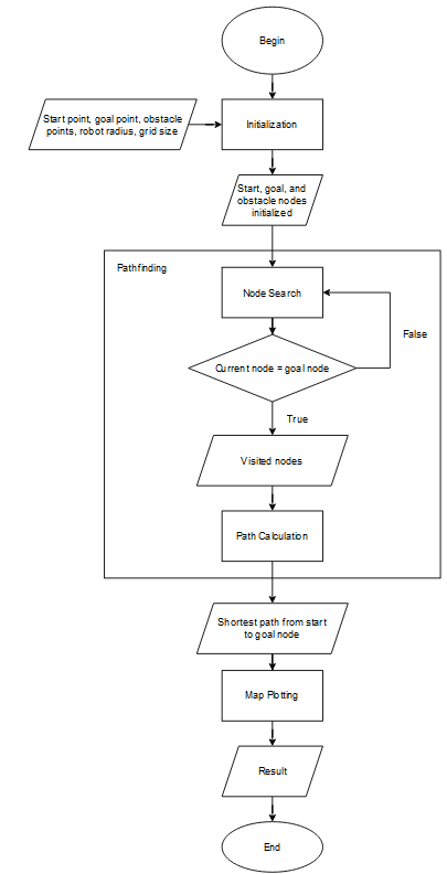
| Figure 3: Flowchart of the program |
The process within the program can be divided into three main steps:
- Initialization
- Path Finding
- Node Search
- Path Calculation
- Map Plotting
The initialization process includes the definition of the Node class with its following methods, variable and constants declarations, and setting up the coordinates for the obstacles (ox, oy), start point (sx, sy), and goal point (gx, gy) relative to the boundaries of the map.
In this scenario, the nodes of a graph is represented as a 1x1 m^2 grid on the map. Each node has 8 possible neighboring nodes on the following directions: up, down, left, right, up left, up right, down left, down right.
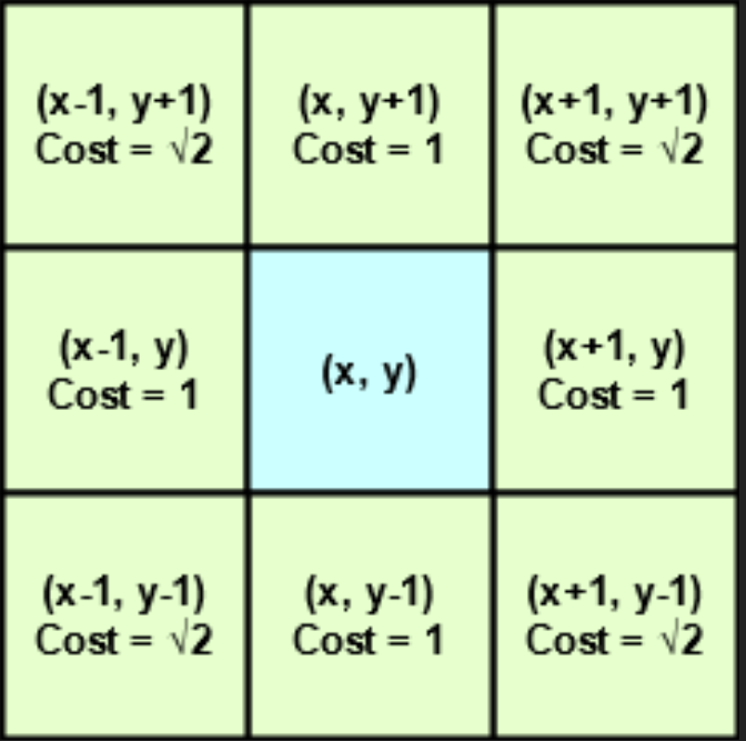 |
|---|
| Figure 4: The possible neighboring nodes (Green) of the current node at (x,y) (Blue) |
To simulate the robot's limited awareness of its surroundings, every grid of the 180x180 m^2 map is not be instantly initialized as nodes at the start. Instead, the program will just start the graph with two unconnected nodes: the start node and the goal node. From the start node, new neighboring nodes will be continually added to the graph as the current node moves from one node to next. The current node will continue iteratively visit the node with the lowest f(n) value. Stored cost value and previous node address of existing nodes will also be replaced if the current cost to the next node is lower.
When the shortest connection is formed in the graph between the start node and the goal node (The current node = goal node), the iteration stops and the program will produce the resulting shortest path.
After the search iteration stops, the program takes the last visited node (The goal node) and iterates back through each previous node's address until it reached. For every node it revisited, the x & y coordinates of each node on the shortest path is stored in its respective result arrays (rx, ry).
The map is plotted using the matplotlib library where obstacles are drawn as a black cirle, start point as a large red circle, goal point as a large magenta circle, and the shortest path as a red line.
The shortest path between the start and goal point is as follows:
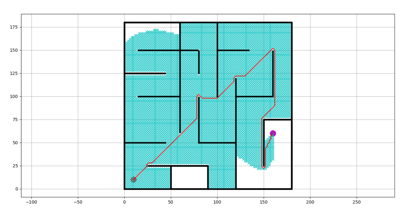 |
|---|
| Figure 5: The shortest path between the start and goal point (Red Line) and the all the visited nodes in the maze (Blue X) |
The program also outputs the following data:
- Number of nodes visited to producte the result: 6398 nodes
- Shortest path distance from start point to goal point: 203.238 m
- Total time: 171.684 s (Results may vary based on machine performance)
The implemented algorithm visited around 78.98% of the total nodes in the map. The performance of the program visibly deteriorated over time as more and more visited nodes are stored and took almost 3 minutes to run on the creator's machine. Based on this data and the results shown in Figure 5, it can be concluded that there is a need to find a more efficient solution than the current implemented algorithm.
Other than the A* algorithm, preliminary tests are done using the D* algorithms that are potentially more efficient than the implemented A* algorithm.
Disclaimer: The test result is done using programs still in development and only serve to highlight potential alternative solutions.
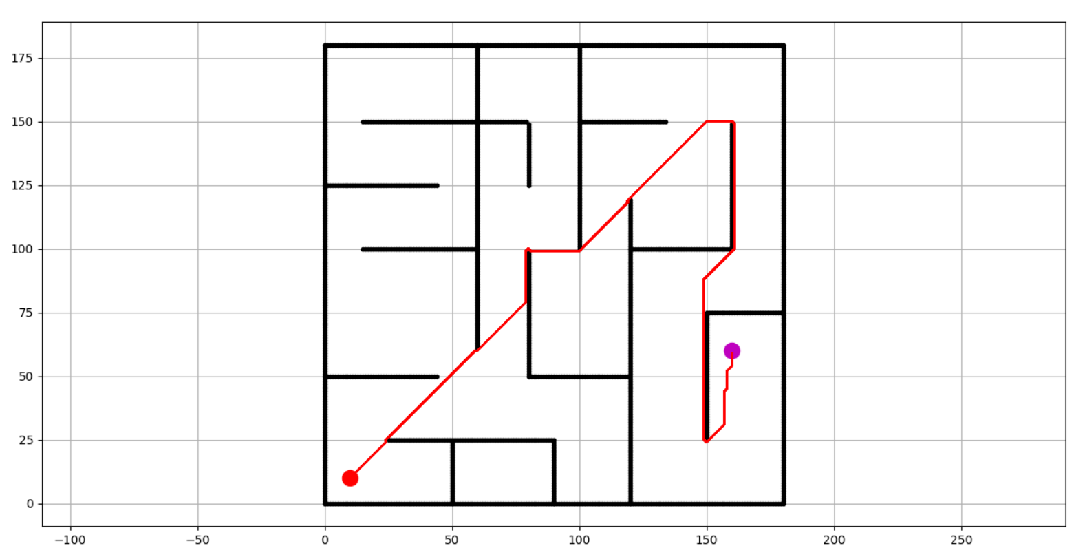
Result of testing using D* algorithm:
 |
|---|
| Figure 6: Test results of implementing the D path-finding algorithm* |
The above result was completed in 14.809 s. Notable issues with this result includes the path being too close to the obstacles, not giving enough room for the diameter of the robot.