04. Array ray tracing using Zemax and Python (an article)
This article describes how to trace large number of rays in Zemax OpticStudio using PyZDDE.
Note: Although the DDE extension has been superseded by the new .NET based extension, Zemax will most likely retain the DDE interface for the foreseeable future.
The array tracing module provides an easy interface to the user for tracing large number of rays as specified in the OpticStudio manual. This module, called arraytrace, is rather independent of the other parts of PyZDDE, and it can be used as a “standalone” module on its own. One can achieve significant speed improvements for tracing large number of rays via extensions using the array ray tracing feature provided by OpticStudio. Figure 1 compares the execution time for tracing a large set of rays using array ray tracing with the total execution time for tracing the same number of rays using single trace per DDE call. We have observed over 200x speed improvements for tracing around 10,000 rays. The factor of improvement in execution time also seems to increase with increase in the number of rays.
The next section briefly explains the interface functions provided by the module. Following the interface section we demonstrate the performance gains we observed in our experiments using array ray tracing. We then provide four examples that demonstrate the use these functions. A short description about the implementation of the array tracing module is provided at the end of the article.
The OpticStudio manual describes five modes of operation for tracing large number of rays. Essentially, array ray tracing involves creating a data structure that specifies the rays and passing it to OpticStudio in a single DDE call. OpticStudio traces the rays and sends the traced data back to the client using the same data structure. For details, please refer to the section “Tracing large number of rays” under the “Extensions” chapter of the manual. The arraytrace module in PyZDDE supports all the five modes of array ray tracing using two core functions and five additional helper functions. They are briefly described here.
The two core functions in arraytrace module are as follows:
-
zArrayTrace()– function for passing an array of ray data structures to OpticStudio -
getRayDataArray()– function to create the ray data structure array (the array of DDERAYDATA structure as described in the OpticStudio manual).
We can use the above two functions in a Python script for tracing rays in any of the five modes. In order to do so, we create the ray data structure array (DDERAYDATA) using getRayDataArray(), fill up the ray data structure array with the appropriate parameters of the rays, and pass the array to OpticStudio using zArrayTrace(). Once the function returns, we need to parse the appropriate data from the array based on the mode. Although the above functions are available to the user, the additional helper functions in the arraytrace module (described below) make the above process easier by hiding the complexity of ray data array creation and parsing. Each of these functions accept ray specifications as Python lists and returns the appropriate traced data as Python lists. The helper functions are as follows:
-
zGetTraceArray()– traces an array of rays defined by normalized field and pupil coordinates, similar tozGetTrace()that traces one ray per DDE call. -
zGetTraceDirectArray()– traces an array of rays defined by the coordinates and direction cosines at a starting surface, similar tozGetTraceDirect()that traces one ray per DDE call. -
zGetPolTraceArray()– for tracing polarized rays defined by normalized field and pupil coordinates, which is similar tozGetPolTrace()that traces one ray per DDE call. -
zGetPolTraceDirectArray()– for tracing polarized rays defined by the coordinates and direction cosines at a starting surface, which is similar tozGetPolTraceDirect()that traces one ray per DDE call. -
zGetNSCTraceArray()– traces a single ray inside a non-sequential group. Rays may split or scatter into multiple paths. The function returns the entire tree of ray data containing split and/or scattered rays.
Please review the examples below to see how the above functions work.
As a measure of performance gain, Figure 1 compares the execution time for tracing large set of rays using array ray tracing with the total time required for tracing the corresponding set of rays that were traced using zGetTrace() (i.e. using a DDE call for every ray) for multiple sets of rays. We have used the standard Cooke Triplet 40 degree field lens file for this experiment. Please note that execution times will vary depending upon the specific system’s hardware and software configuration.
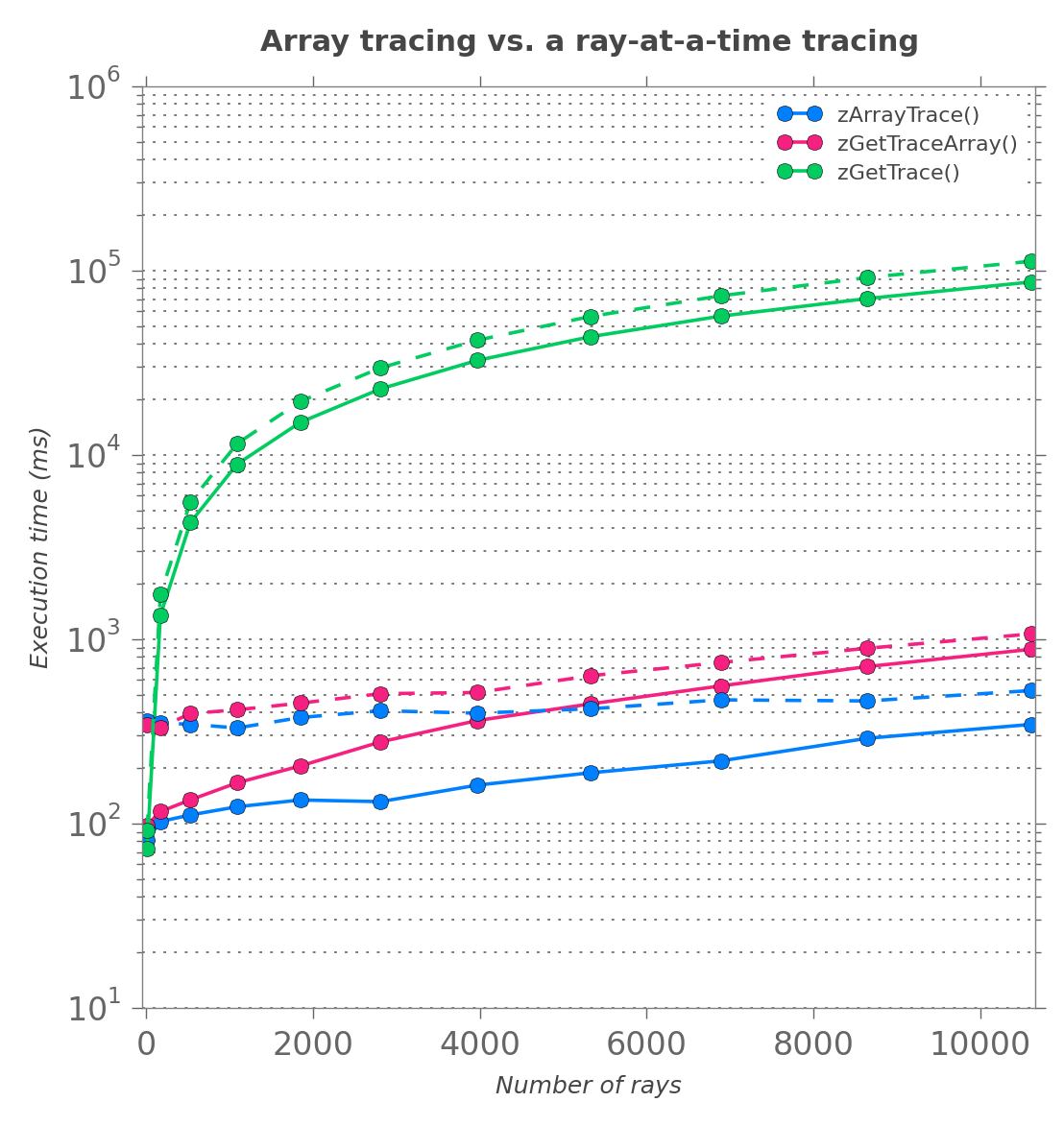
The y-axis, which represents the execution time in milliseconds, is logarithmically scaled. The x-axis denotes the number of rays traced. The solid lines represent the execution times on a 64-bit Win 7 running on 1.30GHz Intel® Core™ i5 (2 physical cores, 4 processors with HTT) with 16.0GB RAM and solid state memory. The dashed lines show execution times on a 64-bit Win 7 running on 1.73 GHz Intel® Core™ i7 (4 physical cores, 8 processors with HTT) with 8.0GB RAM and traditional HDD. The better performance in the dual-core i5 machine over the quad-core i7 machine is (most likely) due to the larger RAM and solid-state memory in the former. zGetTrace() makes a DDE call from Python to OpticStudio for every single ray traced. zGetTraceArray(), which is the array-based equivalent of zGetTrace(), accepts lists of ray parameters, creates the appropriate ray data structure and request OpticStudio to trace the rays in a single DDE call. As described earlier, zArrayTrace() is the core function that passes the ray data structure array to OpticStudio. It is used by zGetTraceArray() and other helper functions such as zGetTraceDirectArray(), zGetPolTraceArray(), etc. in the arraytrace module. The helper functions tend to be are slightly slower compared to zArrayTrace() because of the use of Python lists for passing ray parameters. The plot shows that there is a significant advantage of using array tracing functions for tracing large number of rays. For example, in our experiments, tracing 10609 rays using zArrayTrace() took about 0.53 seconds compared to 1 minute 52 seconds required for tracing the same number of rays using zGetTrace(). That is over 200x improvement in performance. The graph also shows that while the execution time linearly increases with the number of rays for zGetTrace() function (traces a single ray per call), it remains quite steady with increase in the number of rays using the array ray tracing feature. Also, it must be kept in mind that speed is especially not a forte of Python. An extension using pure C-language (e.g. the ArrayDemo.c extension sample that is shipped with OpticStudio) takes under 50 milliseconds to trace 10500 rays. However, code development in Python is much faster, easier, and arguably much less error prone than writing code in C.
Here we present few examples of the array ray tracing functions from the arraytrace module in PyZDDE.
The first example we consider emulates the “ArrayDemo.c” demo provided by OpticStudio. This will also allow us to verify the output of the core function with the reference provided by OpticStudio. Additionally, it demonstrate the use of the two core functions – zArrayTrace() and getRayDataArray(). Note that the arraytrace module is standalone that can be used without creating an explicit DDE link. This is because the zArrayTrace() function creates a separate DDE link for passing and retrieving ray data to/from OpticStudio. The ray tracing is performed on a lens file present in the lens-data-editor (LDE) in OpticStudio. In this example, we use the zdde module only for loading and pushing the lens file into the LDE, which could have been done manually as well. The Python script for tracing 441 rays is shown below. Several of the ray traced data are outputted to a text file called arrayTraceOutput.txt.
from __future__ import print_function, division
import pyzdde.arraytrace as at  # Module for array ray tracing
import pyzdde.zdde as pyz       # PyZDDE
from os import path
from math import sqrt as sqrt

# load Cooke triplet zmx file
zmxfile = 'Cooke 40 degree field.zmx'
ln = pyz.createLink()
filename = path.join(ln.zGetPath()[1], "Sequential\Objectives", zmxfile)
ln.zLoadFile(filename)
ln.zPushLens(1)
numRays = 21**2  # 441 rays will be traced
radius = int(sqrt(numRays)/2)

# create the ray data structure array
rd = at.getRayDataArray(numRays, tType=0, mode=0, endSurf=-1)

# fill the rest of the ray data array
k = 0
for i in range(-radius, radius + 1, 1):
    for j in range(-radius, radius + 1, 1):
        k += 1
        rd[k].z = i/(2*radius)   # px
        rd[k].l = j/(2*radius)   # py
        rd[k].intensity = 1.0
        rd[k].wave = 1

# trace the rays
ret = at.zArrayTrace(rd, timeout=5000)

# write the ray trace data into a file
outputfile = "C:\\tmp\\arrayTraceOutput.txt"
if ret==0:
    k = 0
    with open(outputfile, 'w') as f:
        f.write("Listing of Array trace data\n")
        f.write("{:^7} {:^7} {:^7} {:^15} {:^15} {:^9} {:^9} {:^9} {:^6}"
                " {:^7} {:^7} {:^7} {:^7} {:^7} {:^7} {:^7}\n"
                .format('px', 'py', 'error', 'xout', 'yout', 'l', 'm', 'n',
                        'opd', 'Exr', 'Exi', 'Eyr', 'Eyi', 'Ezr', 'Ezi', 'trans'))
        for i in xrange(-radius, radius + 1, 1):
            for j in xrange(-radius, radius + 1, 1):
                k += 1
                line = ("{:7.3f} {:7.3f} {:5d} {:15.6E} {:15.6E} {:9.5f} "
                        "{:9.5f} {:9.5f} {:7.3f} {:7.3f} {:7.3f} {:7.3f} "
                        "{:7.3f} {:7.3f} {:7.3f} {:7.4f}\n"
                        .format(i/(2*radius), j/(2*radius), rd[k].error,
                                rd[k].x, rd[k].y, rd[k].l, rd[k].m, rd[k].n,
                                rd[k].opd, rd[k].Exr, rd[k].Exi, rd[k].Eyr,
                                rd[k].Eyi, rd[k].Ezr, rd[k].Ezi, rd[k].intensity))
                f.write(line)
else:
    print("There was some problem in ray tracing")
# cleanup and close
ln.zNewLens(); ln.zPushLens()
ln.close()
Here is a partial output from the file arrayTraceOutput.txt:
Listing of Array trace data
 px       py     error       xout          yout           l        m           n     opd      Exr      Exi     Eyr     Eyi     Ezr   Ezi   trans
 -0.500  -0.500     0   -2.985686E-03   -2.985686E-03   0.05014   0.05014   0.99748  64.711   0.000   0.000   0.000   0.000  -1.000   0.000  1.0000
 -0.500  -0.450     0   -3.529811E-03   -3.176830E-03   0.05013   0.04511   0.99772  64.711   0.000   0.000   0.000   0.000  -1.000   0.000  1.0000
 -0.500  -0.400     0   -4.037443E-03   -3.229955E-03   0.05012   0.04009   0.99794  64.711   0.000   0.000   0.000   0.000  -1.000   0.000  1.0000
 -0.500  -0.350     0   -4.501208E-03   -3.150846E-03   0.05011   0.03508   0.99813  64.711   0.000   0.000   0.000   0.000  -1.000   0.000  1.0000
 -0.500  -0.300     0   -4.914870E-03   -2.948922E-03   0.05010   0.03006   0.99829  64.711   0.000   0.000   0.000   0.000  -1.000   0.000  1.0000
We have compared the above output to that produced by “ArrayDemo.c” and found them to match.
The second example is functionally equivalent to the first example, except that we use the zGetTraceArray() helper function. In order to use this function we construct two lists of the normalized pupil position coordinates px and py for the rays (441 rays in total), and pass the lists along with the ray count and wavelength number to the function. After tracing is done, the function returns 13 lists (if the ray tracing was successful) containing the error, vig, x, y, z, l, m, n, l2, m2, n2, opd and intensity for each ray. We then print the result for the first 10 rays. It is also intended to show that the pyzdde.arraytrace module can be used independent of pyzdde.zdde module. Since we are not using the pyzdde.zdde module we cannot load a lens file programmatically. Therefore, this example assumes that a lens file (the Cook triplet 40 degree field in this case) was manually loaded into OpticStudio before executing the program. The example shows how convenient it is to simply call zGetTraceArray() instead of trying to construct the ray data array and retrieve tracing data from the structure after the tracing finished. It also demonstrates the ease with which we can perform array ray tracing in OpticStudio using the external interface.
from __future__ import print_function, division
import pyzdde.arraytrace as at  # Module for array ray tracing
from os import path
from math import sqrt as sqrt

numRays = 21**2  # 441 rays will be traced
radius = int(sqrt(numRays)/2)

flatGrid = [(x/(2*radius),y/(2*radius)) for x in xrange(-radius, radius + 1, 1)
                    for y in xrange(-radius, radius + 1, 1)]

px = [e[0] for e in flatGrid]
py = [e[1] for e in flatGrid]

rd = at.zGetTraceArray(numRays=numRays, px=px, py=py, waveNum=1)

if rd not in [-1, -999, -998]:
    print("{:^7} {:^7} {:^9} {:^5} {:^5} {:^9} {:^7} {:^6} {:^7}"
          .format('px', 'py', 'error', 'x', 'y', 'l', 'm', 'n', 'intensity'))
    for i in range(10):
        print("{:7.3f} {:7.3f} {:5d} {:7.3f} {:7.3f} {:7.3f} {:7.3f} {:7.3f} {:7.3f}"
              .format(px[i], py[i], rd[0][i], rd[2][i], rd[3][i],
                      rd[5][i], rd[6][i], rd[7][i], rd[12][i]))
else:
    print("Error in ray tracing")
Output from the above code:
 px         py    error  x       y       l       m       n    intensity
 -0.500  -0.500     0  -0.003  -0.003   0.050   0.050   0.997   1.000
 -0.500  -0.450     0  -0.004  -0.003   0.050   0.045   0.998   1.000
 -0.500  -0.400     0  -0.004  -0.003   0.050   0.040   0.998   1.000
 -0.500  -0.350     0  -0.005  -0.003   0.050   0.035   0.998   1.000
 -0.500  -0.300     0  -0.005  -0.003   0.050   0.030   0.998   1.000
 -0.500  -0.250     0  -0.005  -0.003   0.050   0.025   0.998   1.000
 -0.500  -0.200     0  -0.006  -0.002   0.050   0.020   0.999   1.000
 -0.500  -0.150     0  -0.006  -0.002   0.050   0.015   0.999   1.000
 -0.500  -0.100     0  -0.006  -0.001   0.050   0.010   0.999   1.000
 -0.500  -0.050     0  -0.006  -0.001   0.050   0.005   0.999   1.000
The usage pattern of the helper functions zGetTraceDirectArray(), zGetPolTraceArray(), and zGetPolTraceDirectArray() are very similar to zGetTraceArray().
In our next example, we explore the fifth mode of array ray tracing, which is provided by the function zGetNSCTraceArray(). This mode is used for tracing rays inside of a non-sequential group. It is different from the other modes in that only one ray is specified to the function; however, the ray may split or scatter into multiple paths and the function returns the entire tree of ray data. The example considered below is a Python version of the example “NSCTraceDemo.c” provided by Zemax (found in C:\Program Files\Zemax OpticStudio\Extend). It assumes that a NSC model is pre-loaded into OpticStudio. For this example, the model “Example 3 Grating Splits up Color.zmx” (from …\ZEMAX\Samples\Non-sequential\Colorimetry) was used.
from __future__ import print_function, division
import os as os
import pyzdde.arraytrace as at
import pyzdde.zdde as pyz

ln = pyz.createLink()
ln.zGetRefresh()
zmxfile = os.path.split(ln.zGetFile())[1]

# Get maximum number of segments
maxSeg = ln.zGetNSCSettings().maxSeg

# limit the number maximum number of segments to 50
nMaxSeg = maxSeg if maxSeg < 50 else 50

# Trace a single in NSC mode with polarization and splitting, but no scattering.
rayData = at.zGetNSCTraceArray(n=1, Eyr=1.0, intensity=1, surf=1, usePolar=1,
                               split=1, nMaxSegments=50)

# Print the output
print("Listing of NSC Trace data:")
print("{:^4} {:^4} {:^4} {:^6} {:^4} {:^14} {:^14} {:^14} {:^12}"
      .format('seg#', 'Prnt', 'Levl', 'In', 'Hit', 'X', 'Y', 'Z', 'Intensity'))

totalSegments = len(rayData)
for i, seg in enumerate(rayData):
    segLevel = seg.segment_level
    segParent = seg.segment_parent
    insideOf = seg.inside_of
    hitObj = seg.hit_object
    x, y, z, l, m, n = seg.x, seg.y, seg.z, seg.l, seg.m, seg.n
    intensity = seg.intensity
    opl = seg.opl
    print("{:4d} {:4d} {:4d} {:4d} {:4d} {:15.6E} {:15.6E} {:15.6E} {:8.4f}"
           .format(i+1, segParent, segLevel, insideOf, hitObj, x, y, z, intensity))

ln.close()
Output from running the above code:
Listing of NSC Trace data:
seg#   Prnt     Levl    In    Hit       X               Y              Z          Intensity
   1      0       1      0     2    0.000000E+00    0.000000E+00    5.000000E+00   1.0000
   2      1       2      2     2    1.435769E-01    0.000000E+00    5.500000E+00   0.3300
   3      2       3      0     3    4.307306E+00    0.000000E+00    2.000000E+01   0.3300
   4      1       2      2     2    0.000000E+00    0.000000E+00    5.500000E+00   0.3300
   5      4       3      0     3    0.000000E+00    0.000000E+00    2.000000E+01   0.3300
   6      1       2      2     2   -1.435769E-01    0.000000E+00    5.500000E+00   0.3300
   7      6       3      0     3   -4.307306E+00    0.000000E+00    2.000000E+01   0.3300
   8      1       2      0     0    5.520000E-01    0.000000E+00    3.077685E+00   0.3300
   9      1       2      0     0    0.000000E+00    0.000000E+00    3.000000E+00   0.3300
  10     1       2      0     0   -5.520000E-01    0.000000E+00    3.077685E+00   0.3300
Again, we have compared the above output to that produced by “NSCTraceDemo.c” and found them to match.
The last example shows how the array ray tracing module provides handy functionality in assessing the performance of an optical system. This example makes use of NumPy and Matplotlib, which are two common Python packages in scientific computation. Please refer to the implementation for more information.
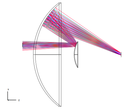
Figure 2 shows a simple two mirror configuration derived from a schwarzschild system. While the system is conceptually very simple (just two mirrors), it has an asymmetric field, and the spots vary significantly over the field. This is because it is an off-axis imaging system.
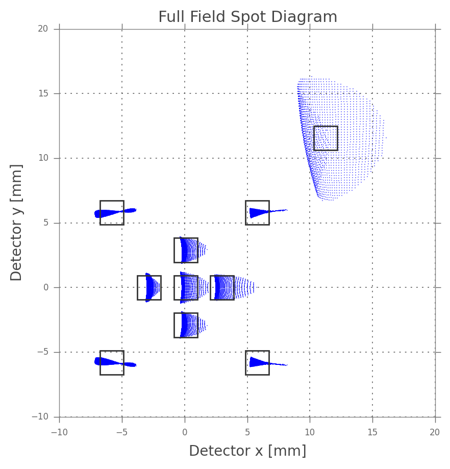
A custom Full Field Spot Diagram generated using the arraytrace module is shown in Figure 3 for a set of pre-defined fields. All the spots are shown on a single 2d plot. While the xy position of each spot is shown according to the actual position on the image plane, the magnification of each spot can be chosen for best visual appearance. For reference, a box of 25x25 microns is shown for each spot. The deformation of the spots over the field-of-view is clearly seen. This plot is very similar to the inbuilt “Full Field Spot Diagram” of OpticStudio.
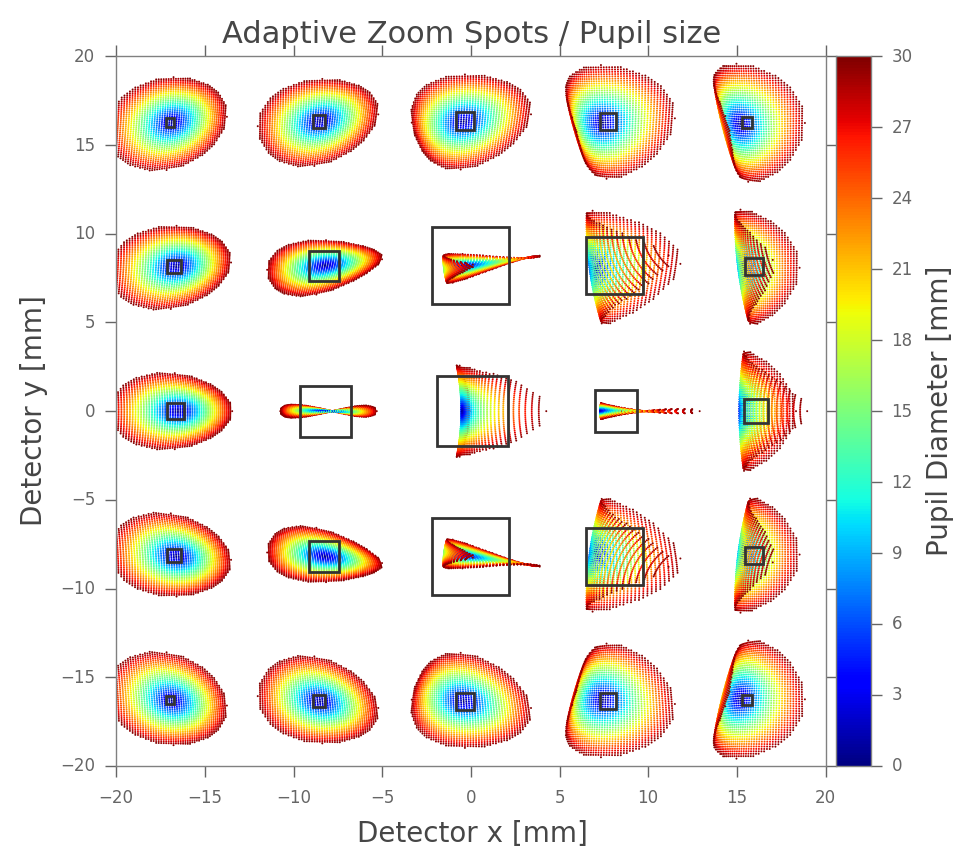
We can create more fancy plots based on a certain need. For example, in Figure 4 we generate a grid of NxN field points and use array tracing to create spot diagrams for all field points on a single 2d figure. However, this time the magnification of each spot is adapted to its RMS radius. Again, for reference, the box shown on each spot is 25x25 microns. Furthermore, the rays in the spots are color coded by their radial pupil coordinate. We can immediately observe how the spots shrink/ grow with decrease/ increase in size of the aperture stop.
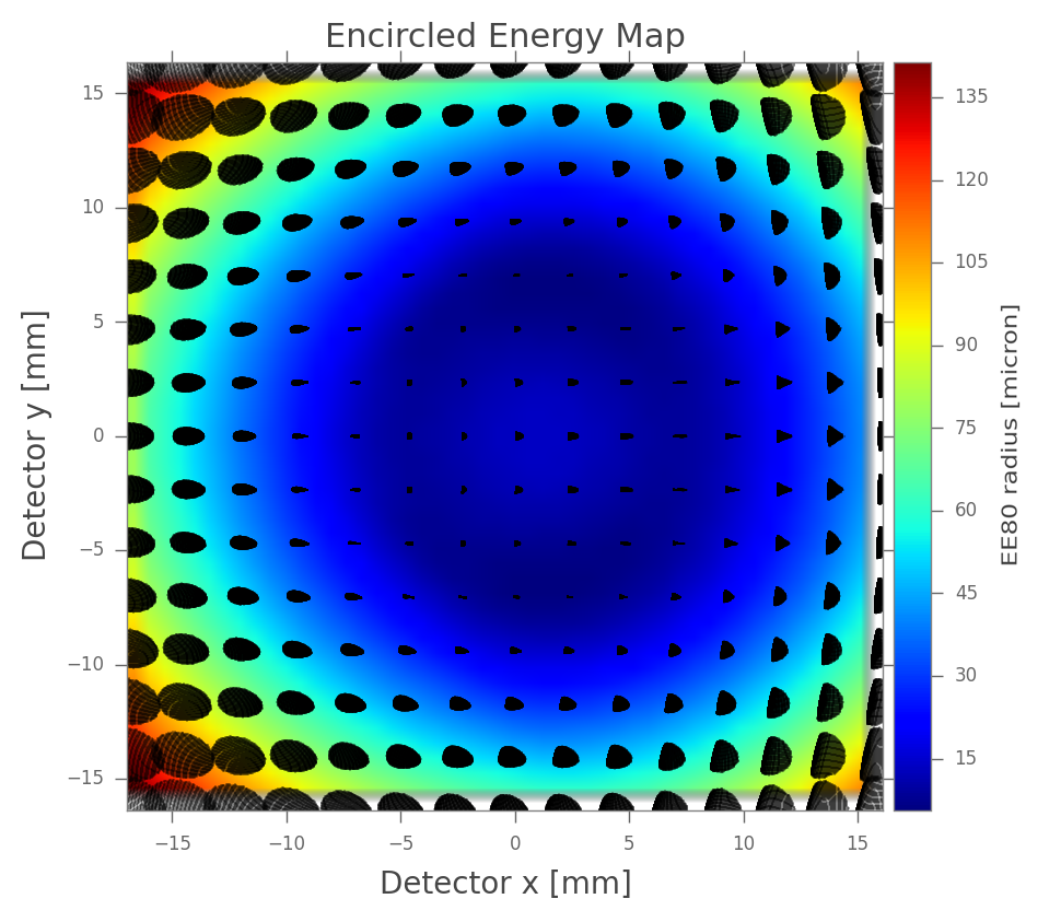
The last plot demonstrates how a denser grid of spot diagrams over the whole field can be used to generate encircled energy (EE) maps or RMS spot size maps. Figure 5 shows the radius of the spots in microns where 80% of the rays lie within. This can easily be adapted to calculate the EE within one pixel of a detector if desired. The plot was generated by calculating spot radii for a dense grid of spots over the field and interpolation. The spots that have been used for calculating the radii are shown as an overlay to the plot. Producing such plots by tracing one ray per DDE call would require enormously large amount of time. Generating all the plots in this example took about 12 seconds on average in our test computer which has just 8 GB RAM.
It should be emphasized that the general procedure – generate spot diagrams via the arraytrace module and plot them on a common canvas – also works for different configurations and/or wavelengths by simply adding a loop over the appropriate variable (configuration / wavelength). Therefore, the method also works for more complex optical systems such as spectrographs where the defined wavelengths depend on the configuration.
A more extensive repository of examples can be found within the “Examples” directory of PyZDDE. Few examples that demonstrate a specific aspect of the array ray tracing module (arraytrace) may be found at Array ray tracing examples.
Zemax provides a C-language reference implementation of a DDE client, called "zclient.c". The current version of the arraytrace module was created using ctypes to wrap a modified version of "zclient.c". As a result, the array tracing module is really a standalone module. Unlike the other features of PyZDDE, the user is not required to establish an explicit DDE link object to communicate with OpticStudio as it was demonstrated in the second example above.
As PyZDDE aims to use modules only from the standard Python library, NumPy was deliberately not used in arraytrace module. However, if desired, the user can use NumPy arrays to create the ray data structure array and pass it to OpticStudio using the function zArrayTrace(). Another option is to convert the NumPy arrays to lists (e.g. using the tolist() method) before passing the arrays to the helper functions for array ray tracing as demonstrated in the fourth example in this article.
At the time of this writing, emphasis was given to the correctness of the function rather than performance. Future versions may have improved performance.
We introduced the arraytrace module of PyZDDE, and demonstrated that we can expect large performance gains when tracing large number of rays using the array tracing feature provided by OpticStudio. We have also shown that it is relatively easy to setup and execute array tracing using the helper functions in the module.
The authors would like to thank Ian Rousseau for discussions and initial implementation ideas about the array ray tracing module.
This article is authored by Indranil Sinharoy, and Julian Stuermer.
This work by PyZDDE contributors is licensed under a Creative Commons Attribution 4.0 International License.
Based on a work at https://github.com/indranilsinharoy/PyZDDE.
