Welcome to the fourth article in this series where we’re diving deep into Neural Networks.
In this article, we’re discussing PyTorch’s efficiency and performance when challenged with different parameters, and how these parameters can effect the training time of a model.
From a popularity perspective, I’ve extracted this information from Google Trends to analyze the popularity of PyTorch and Tensorflow :
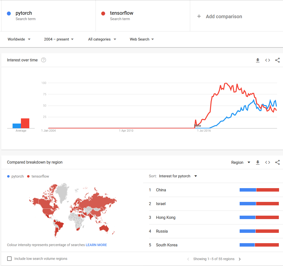
As we can see, TensorFlow is reigning right now over the world. Let’s see if performance matches expectations.
For conducting these tests, we need to ensure that the hardware on which we test has the same specifications as in the next article, where we’ll analyze TensorFlow’s performance.
Additionally, it’s recommended to perform tests in private/dedicated infrastructure, meaning that we’d ideally need:
- Dedicated infrastructure instead of using shared infrastructure — This means that it’d be ideal to have an OCI Compute Instance being given to you and no one else. This prevents the CPU, for example, from virtually sharing resources with other OCI users. This will in turn reduce I/O interruptions which will make our benchmarking tests much more accurate.
- One shared notebook session — so that the Operating System doesn’t accidentally give more priority to one Jupyter / Zeppelin project than the other through the CPU scheduler.
The machine specifications for this test are:
- OCI Compute Shape: VM.Standard.E3.Flex. This is a great shape and probably one of my favorite as it allows us to choose a variable number of CPUs / DRAM (up to 100 OCPUs).
- Number of OCPUs: 16
- Amount of memory (GB): 32
- Block storage size (in GB): 100. We won’t need that much, but it’s the minimum amount that we can choose in OCI. When we use OCI Data Science, we can create a notebook session with up to 10,240 GB (10TB), should you ever need that much for your use case.
I’ve chosen to run with a CPU version, unlike previous articles where I used a GPU instance, just to save myself some money. If you’re interested in finding out the specifics of drastically improving your GPU throughput, let me know and I’ll make sure to write something about it in future articles.
To increase the baseline performance of any model, we also need to consider what we’re competing against. Surely, it’s great to create our own model with a couple of layers and see our work being put under pressure against some datasets. But I believe the beauty of data science, and also the most difficult part, is knowing where to look for something better, perhaps by someone with more experience. Let’s face it: there’ll always be someone better than us at anything we’ll ever try, so why not take advantage of this fact? The Internet allows us to look for better things, constantly.
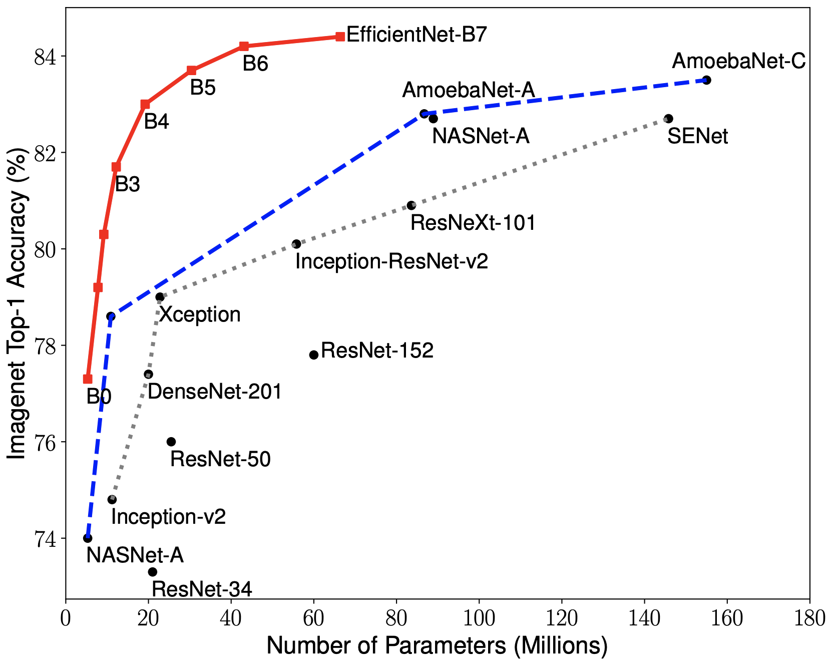
For measuring PyTorch's performance, we'll use a deep Neural Network called EfficientNet, which has been tested against several image processing datasets. It’s a pre-trained convolutional neural network which attempts to systematically change how people approach design and architecture of their own models. In this case, EfficientNet focuses on applying its own specific scaling throughout all dimensions of an image (depth, width, resolution) using a coefficient called C. Using this coefficient has been proven to work pretty well (one of its variants, called EfficientNet 7 has the highest accuracy ever on the ImageNet dataset), being about 8 times smaller than other models in the top list (and being about 6 times quicker). Aside from being able to predict results accurately against the ImageNet dataset (which could be considered an extremely difficult task by itself), it performs very well on other commonly known datasets such as CIFAR100, a dataset that contains images of animals, the Flowers dataset and three other datasets; with many less parameters than the model's competitors.
Think of EfficientNet models as the automation of the design and architecture part of NNs. This automation is super helpful, not just for our specific use case, but in several image processing problems that you’ll find in your career as a data scientist,data analyst, or similar role.
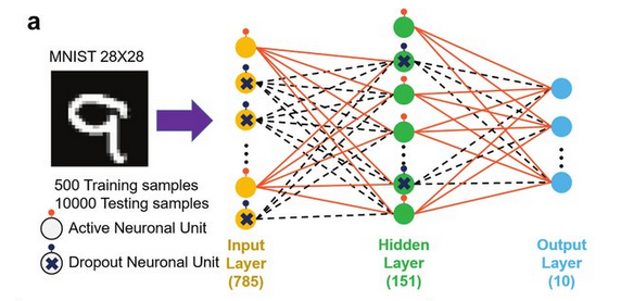
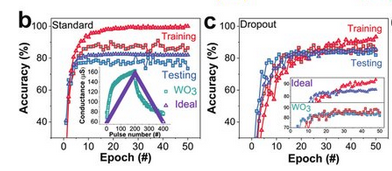
EfficientNet uses millions of parameters, and can therefore be considered a deep Neural Network. I wanted to mention the effect that the Dropout layer (which we applied in last article) can have on significantly improving the accuracy of an NN. Here, we can graphically observe the effect of a Dropout layer when implemented by looking at which neurons are activated and which ones are deactivated and how this hidden layer implementation attempts to reduce the noise created by inaccurate predictions, subsequently increasing the train/test accuracy of the model. Sample images were measured using the MNIST dataset:
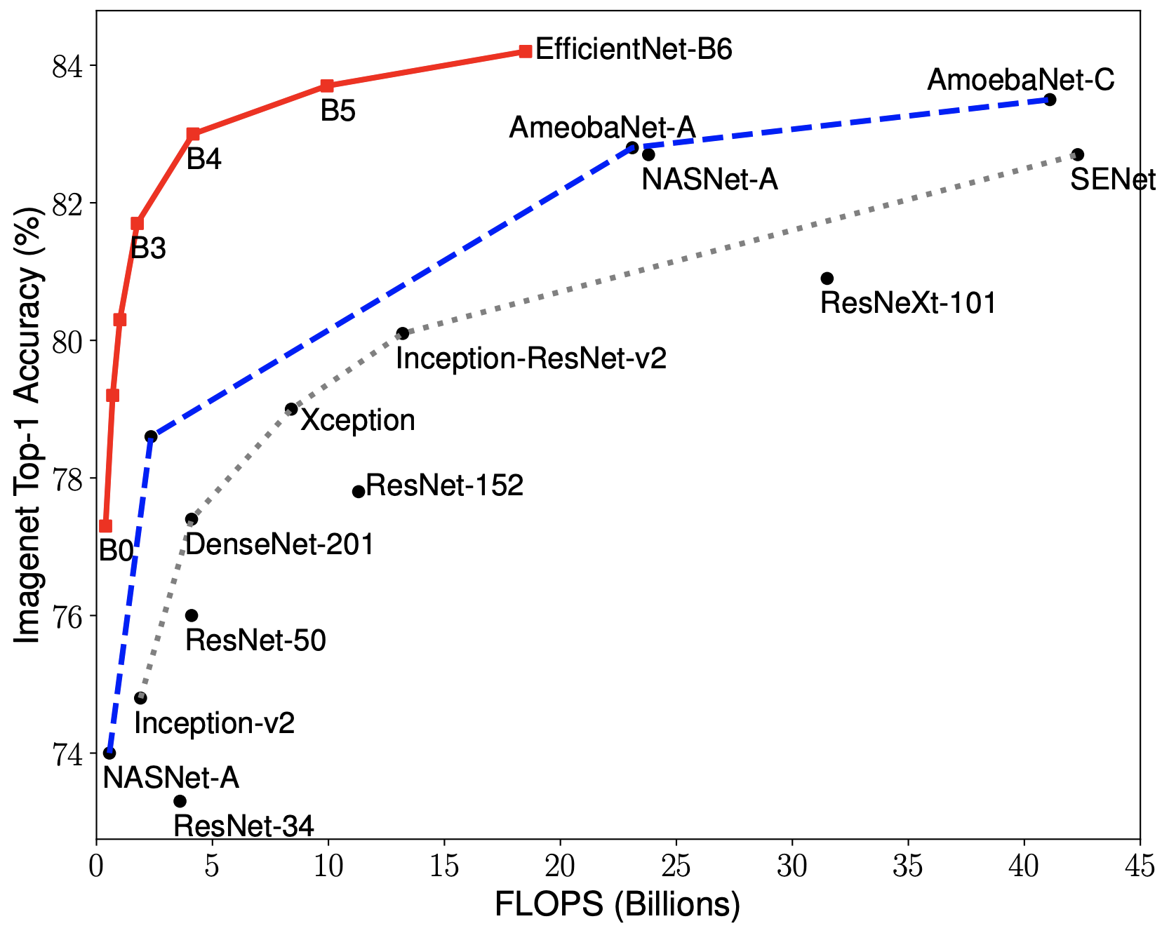
One can argue that EfficientNet is a “simple” model, but in reality we need to consider that, since training is done automatically by computers, millions of operations are performed every second, which causes models like this to have millions of parameters. I took some visualizations from the original TensorFlow repository (which has some documentation about EfficientNet) and displayed it here for you, so you can have a sense of "size" of models such as this one; and to give you a perspective of how well EfficientNet's new coefficient C is compared to other models.
The first image considers the number of parameters in millions, compared to other models. The second image compares the number of floating point operations performed by the models to make predictions.
There are several options to perform a benchmark. Of course, we can always use the standard libraries offered by Python to help us with this, or choose a more advanced approach like PerfZero. In this case, we’re going to avoid complicated libraries, as learning how to perform a benchmark in a correct way is more important than learning how to use a specific library / tool. As technology changes, I’ll always say the most important thing is to mentally return to fundamental concepts and basic ideas in our minds, and then delve into exploring and trying specifics if we need them in our use cases.
So, to create this article I've tested a very beginner-friendly package that I found from PyPi called pytorch-benchmark, and a standard time measurement. Props to Lukas Hedegaard for the great package.
First of all, we install the library:
pip install pytorch-benchmarkWe load our necessary modules into the code:
import numpy as np
import torch
import torch.nn as nn
import datetime
from torchvision.models import efficientnet_b0, efficientnet_b1 # b0...b7
from pytorch_benchmark import benchmark # benchmarking library
We create our function which will perform the benchmark
import yaml

def benchmark_efficientnet():

    model = efficientnet_b0() # change to whichever model you want to benchmark its performance
    # also, I discovered it's possible to perform benchmarking to your own custom models.
    # check this URL out from Lukas Hedegaard: https://github.com/LukasHedegaard/pytorch-benchmark/blob/main/tests/test_custom_class.py

    if torch.cuda.is_available():
        model = model.cuda()

    sample = torch.randn(2, 3, 224, 224)  # (B, C, H, W)

    results = benchmark(
        model=model,
        sample=sample,
        num_runs=1000,
        batch_size=8,
        print_details=True
    )

    for prop in {"device", "flops", "params", "timing"}:
        assert prop in results

    return yaml.dump(results)
Warming up with batch_size=1: 100%|██████████| 1/1 [00:00<00:00, 21.34it/s]
Warming up with batch_size=1: 100%|██████████| 10/10 [00:00<00:00, 30.06it/s]
Measuring inference for batch_size=1: 100%|██████████| 100/100 [00:03<00:00, 32.58it/s]
Warming up with batch_size=8: 100%|██████████| 10/10 [00:01<00:00, 8.05it/s]
Measuring inference for batch_size=8: 100%|██████████| 100/100 [00:11<00:00, 8.50it/s]And we use the library to help us measure performance.
result = benchmark_efficientnet()
print(result) # beautify it
After executing the function, we see the output (very long in our case). The benchmarking flow goes as follows (picture taken from Lukas Hedegaard's GitHub):
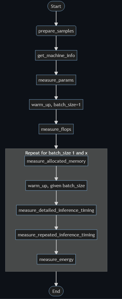
Our EfficientNet model has 5.29 million parameters, and we can see the different steps.
Like in all modern Convolutional NNs (CNNs), the structure followed in EfficientNet models (how they're built on the inside) is as follows:
- A convolution (basically, dividing the image into smaller pieces so that the NN can try and learn about each part of the image separately)
- A batch normalization (BatchNorm2D)
- An activation function, in this case SiLU (we saw ReLU before, the difference can be seen in the picture below)
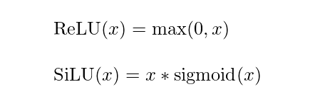
This process is usually repeated several times and mixed with other blocks (like squeeze-and-excitation (SE) blocks). Don’t panic when you hear these terms! They’re just fancy ways to improve the performance of the model internally. You’re free to check out the paper on SE blocks if you want.
This is done many times in the process, and each time we see how the model has considered more/less parameters in each one of the layers of the CNN.
Additionally, at the end of the file, we have a lot of device information. Note that we weren’t able to extract the amount of allocated DRAM as these things are only available when executing benchmarks in machines that support and use the CUDA architecture. Similarly, we can’t gather energy consumption statistics as this is officially only supported for NVIDIA Jetson devices.
Here's a bit of information about the execution:
- MFLOPS (millions of floating operations per second): ~401
- Used DRAM: 3.56 GB
- Average batches per second (batch size = 1) in [27.01, 42.20]
- Average batches per second (batch size = 8) in [18.06, 27.73]
- Batch latency (batch_size = 1) in [23.697, 37.018] ms
- Batch latency (batch_size = 8) in [36.067, 55.365] ms
As expected, the performance when making calculations in batches of 1 is greater than in batches of 8. However, we can clearly see that it isn’t 8 times greater, which means that using batches is actually beneficial.
Note that the batch latency represents the metric we're most interested in, which is how long it takes for one row of data / sample to traverse the neural network at the same time.
As we can see, it wasn't so hard to benchmark the performance of the EfficientNet model using PyTorch.
Considering our machine specs, with 16 Intel(R) Xeon(R) Platinum 8167M @ 2.00GHz OCPUs, we yield 0.28ms / OCPU / row of data.
Also, 401 MFLOPS were calculated in a span of:
- For batch size = 1: 26 seconds
- For batch size = 8: 42 seconds
This means about 15.4 MFLOPS / second, which also yields ~0.96 MFLOPS / second / CPU.
In the next article, we’ll run a similar exercise with TensorFlow with the hope of trying to compare both libraries, and test the hypothesis we formulated in previous articles about TensorFlow being a bit “slower” due to the Keras ecosystem being used on top of TensorFlow itself.
I've attached the notebook with the code used in this article in case you're interested in downloading and trying yourself.
Stay tuned...
Remember that you can always sign up for free with OCI! Your Oracle Cloud account provides a number of Always Free services and a Free Trial with US$300 of free credit to use on all eligible OCI services for up to 30 days. These Always Free services are available for an unlimited period of time. The Free Trial services may be used until your US$300 of free credits are consumed or the 30 days has expired, whichever comes first. You can sign up here for free.
If you’re curious about the goings-on of Oracle Developers in their natural habitat, come join us on our public Slack channel! We don’t mind being your fish bowl 🐠
Written by Ignacio Guillermo Martínez @jasperan, edited by Erin Dawson
Copyright (c) 2021 Oracle and/or its affiliates.
Licensed under the Universal Permissive License (UPL), Version 1.0.
See LICENSE for more details.